Next-generation fault detection for commercial building HVAC systems
Introduction
Modern commercial buildings are becoming more complicated as the number of sensors, actuators and control loops increases. The building management system (BMS) used to control these components will often generate equipment faults and anomalous behaviour, which causes energy waste, thermal discomfort, and drives up maintenance costs. Such system failures may last for a long time before a facility manager or technician notices them. This necessitates the use of automated fault detection and diagnostics (AFDD) tools to detect operational faults and identify their root causes to ensure fault-free operation.
Commercially available analytical software tools typically use a rule-based fault detection and diagnosis (FDD) approach. Rule-based methods are often specific to certain equipment or systems, and their associated control logic. Without proper configurations and continual refinement of the rule sets, a rule-based FDD tool is likely to produce an excessive number of alerts, many of which are related to detected faults trigged by fine-grained rules, but these faults may have an insignificant impact at a building level. The false alerts would also cause the facility manager or maintenance technician to become fatigued and disengaged1.
As buildings become more data-intensive, analytics based on statistical approaches developed for identifying faults and optimisation opportunities has become an active topic within the building energy research community. Statistical FDD methods look at the systems’ measured inputs and outputs and flag faults if differences are statistically significant or exceed a threshold. Statistical approaches have been applied to detect faults for HVAC components such as variable air volume (VAV) boxes2, air handling units (AHUs) 3 and chiller systems4.
They have also been applied to detect faults at a whole-building level 5. Despite all the research effort, no field studies that use data-driven approaches for whole-building fault detection have been reported in the literature.
In this study, we present a novel model-based anomaly detection method based on a statistical approach. The objective is to identify materially significant system anomalies that impact the whole-building energy consumption. At the whole-building level, we apply a random forest (RF) regressor model to map correlation between weather, occupancy level, calendar effects and interval metering data. The model predicts the expected energy usage by using the independent input variables, and then passes it to a search engine to find “best performance on comparable days” (target days) and uses it as a benchmark to detect anomalies at the building level. At the sub-system level, we use the BMS data and technical specification to build sub-models to estimate the energy consumed by each key HVAC component. If a building’s energy use exceeds the target consumption by an amount considered to be statistically significant, the system will navigate down through the hierarchy and find the most probable solutions to close the gap. The outputs of the algorithm include most significant anomalies to be investigated and their corresponding root cause analysis. The proposed method has been field-tested across 10 office buildings, with significant savings achieved during the period of the trial.
Methodology
Structure of model-based anomaly detection
AFDD can be approached by either a bottom-up method or top‑down method 6, 7. In the bottom-up approach, performance states of HVAC subsystems, such as zone temperature, pressure, flow, etc., are investigated to detect issues and propagate their effects on building performance. The disadvantage of this approach is that it may pick up issues that are not important for energy efficiency.
Conversely, in the top-down approach, the detection and diagnostics start with flagging energy increases by the building and subsystems (e.g., electricity consumption, cooling/heating systems), which are measured indirectly by monitoring the amount of electricity or gas provided to the building (or subsystem). The top-down approach is selected if the goal is to achieve energy efficiency.
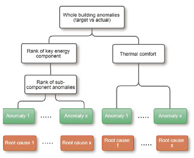
We apply a top-down diagnostic process in this study. The structure of the proposed model-based anomaly detection is illustrated in Figure 1. The workflow is described below. For a given day (actual day) that we wish to find anomalies for, we:
Discover root causes (e.g., economy damper not used) that explain the system anomaly.
- Build a machine learning model that uses weather and interval metering data to find the “best performing comparable day” (target day) over a given historical window.
- Compare the actual day’s interval meter data to the target day to identify anomalies that affect whole-building consumption (for example, energy spikes, higher baseload, and significant daily energy increase).
- Use BMS data and technical specifications of equipment to estimate the energy usage of individual HVAC components (referred to as “soft meters” in this paper).
- Rank the key energy components: Component usage ranking (for example, soft meter chiller total, soft meter AHUs total) based on the difference between actual day and identified target day.
- Rank anomalies at the sub-component level (for example, AHU‑1, Chilled water pump-2) based on the difference between the actual day and comparable day.
- Discover root causes (e.g., economy damper not used) that explain the system anomaly.
Detecting building level anomaly based on target
When performing building energy modelling, it is assumed that a building’s energy performance characteristics do not change during the training period, and weather inputs can be used as independent variables. However, for buildings that are continually being fine-tuned, the energy performance may improve, leading to the possibility that models trained off historical data may over-predict demand. Similarly, a model could under-predict a building’s energy performance if a building’s performance is trending negatively due to the existence of system faults.
To solve this problem, we built an algorithm to identify “target performance” of the building for any given day and use it as the benchmark for anomaly detection. A detailed description of a statistical approach to generate the target is presented in For building operators, what difference does a target make? by A.C. Roussac and H. Huang8. The target performance represents the best performance a building has achieved for a given period under similar weather and occupancy conditions. In our previous study 9, we found that an RF regressor provides the best balance between accuracy and computational speed when used for building energy modelling. Therefore, the RF has been used to search for the target performance in this study. An outline of the algorithm is as follows:
- Obtain historical data with 15 minutes interval from the database and prepare in a format that can be used for training.
- Remove outlier days, weekends and public holidays from the training set.
- Split the data into training and test sets and feed the inputoutput data into the random forest regression for model training.
- Apply cross validation to find the most optimised combination of hyperparameters, e.g., number of trees in the forest, to avoid overfitting.
- Obtain daily prediction within the training period and store them in the database.
- Apply iterative rules to find comparable days that are similar to the day of interest in terms of weather conditions and daily prediction.
- Once the algorithm finds a pool of comparable days with similar weather conditions and model predictions, the algorithm stops searching.
- From the pool of comparable days, find the days that use the minimum amount of energy.
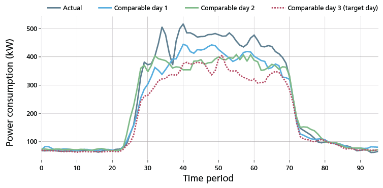
The above algorithm is designed to find the day in the building’s performance history where the minimum amount of energy was used compared to other days with similar weather conditions, i.e., the day that had the best performance under comparable weather conditions. Figure 2 illustrates how the target profile works. The graph shows that our algorithm has picked up three comparable days, but only “Comparable day 3” was selected as the “target day” because it consumed the least energy among the three comparable days.
Simplified energy model for HVAC components
Once an anomaly is detected at the building level, the next step is to find which sub-component contributes most to the energy increase. To achieve this, we build soft meter models, based on the first law of thermodynamics to estimate energy consumption of individual HVAC components.
Chiller model
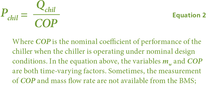
Chillers are the most important components in an HVAC system in warm climates, not only because the chiller is the most energyintensive HVAC component, but also because it has complicated dynamics. Accurate modelling of chiller consumption requires technical details and extensive good‑quality BMS data points. The chiller energy model can be simply expressed as:

The chiller power consumption can then be estimated as:

Fan model
Fan power can be approximated as a second-order polynomial function of the total supply air mass flow rate driven by the fan, and the supply air mass flow rate by the fan determined by summation of airflow to each room. This can be expressed as:

Pump model
When estimating the energy usage of the pumps, it is assumed that the enthalpy change of water through the pumps is constant. It is also assumed that the pump volumetric water flow, the pump speed, and pressure difference generated by the pump satisfy the following equations:
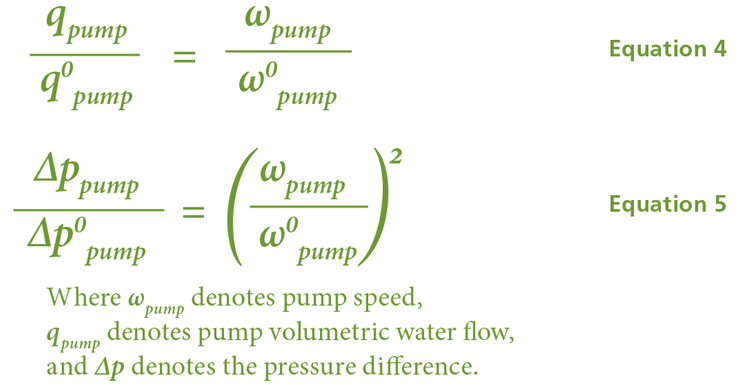
Under the above assumptions, the pump consumption can be calculated using the following equation:

Detecting anomalies at the component level
To estimate the savings potential attributable to each component, we demonstrate two statistical approaches in this study: target deviation analysis and peer group analysis. With the target analysis approach, the targeted expected energy usage of individual components is identified and compared to the actual usage. The deviation is calculated using:

Once the deviation is determined, thresholds can be applied for detecting different levels of anomalies. For sub-components, a wider uncertainty buffer zone of 10% is applied to account for the errors generated by soft meter modelling:

Figure 3 illustrates anomaly detection results by applying the target deviation approach to all the AHU sub-components in an HVAC system. The sub-components include the variables such as cooling valve opening level (AHU_CCV), AHU fan speed (AHU_SPD), and cooling tower fan speed (CT_SPD). Each dot represents the change of usage between actual day and target day. In this graph, the red dots indicate “increase in usage”, the blue dots indicate “neutral”, and the green dots indicate “decrease in usage”. From this graph we can see AHU- 19-2_CCV, AHU‑2‑2_ CCV, and AHU-5-1_CCV are the most anomalous components because they have the largest increase. The straight fitted line illustrates the components that meet the target operation.
Detecting anomalies at the component level
To estimate the savings potential attributable to each component, we demonstrate two statistical approaches in this study: target deviation analysis and peer group analysis. With the target analysis approach, the targeted expected energy usage of individual components is identified and compared to the actual usage. The deviation is calculated using:
| Component name | Identified anomalies | Action items |
|---|---|---|
| Chillers 1 and 3 | Inefficient chiller staging control. | Increased chiller staging delay time from 5 mins to 20 mins |
| AHU 13-1 and AHU 5-2 | AHU fan was running at 100% all the time | Removed vague terminal box out of cooling calculation. |
| AHU-6 | Economy damper was used when OA was too warm | Found the outdoor air damper was overridden to 100% open. |
| AHU-4 | 4 Unnecessary operation | Altered the operational schedules. |
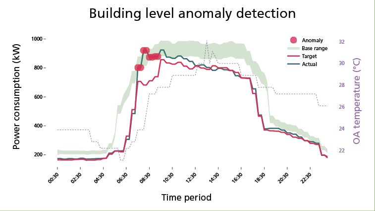
Figure 4 compares the actual electricity profile with the target electricity profile at a whole-building level. It shows that the actual usage on the subject day was ~7 per cent higher than the target consumption. The algorithm identified that the most anomalous period of the day happened from 7am to 9am. We can observe a spiky usage from the actual meter readings during this time, while on the target day, the energy usage in the morning looked much smoother.
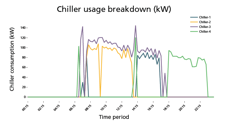
A comparison of chiller consumption is illustrated in Figure 5(a). It clearly shows that the chillers were running harder from 7am to 9am on the subject day compared to the target day, which explains the energy spike that occurred at the whole-building level. Figure 5(b) displays the operational status of different chillers on the investigated day.
After comparing the actual day’s chiller staging with the target, we found that both chillers 2 and 3 were running from 7am to 9am on the investigated day, while on the target day, it was only chiller 1 running. This was later confirmed to be caused by an inefficient chiller staging control strategy. The chiller staging control was then optimised by prolonging the chiller staging delay time and increasing the minimum chilled water temperature set-point.
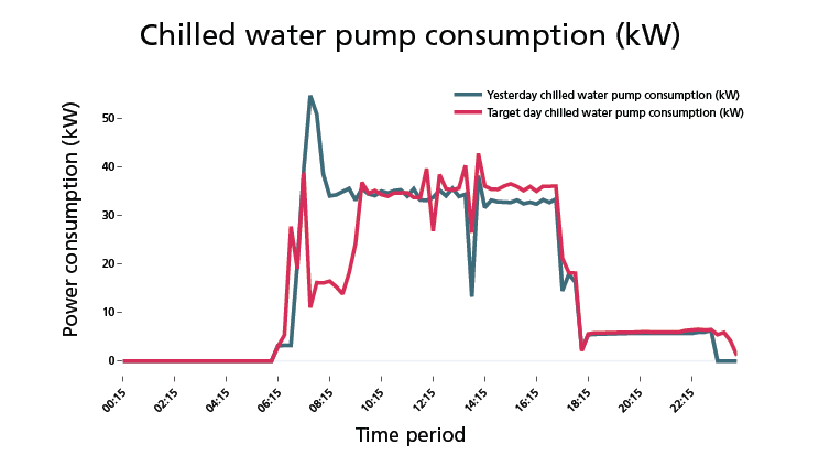
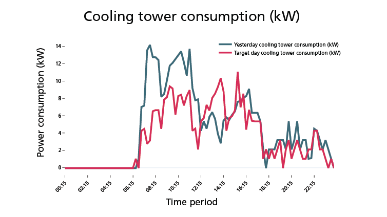
Further, from Figure 6 (a) and (b), we can see chilled water pump and cooling tower fan profiles also show morning spikes, which are tied up to the chiller staging issue.
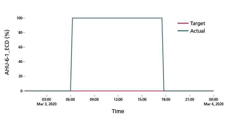
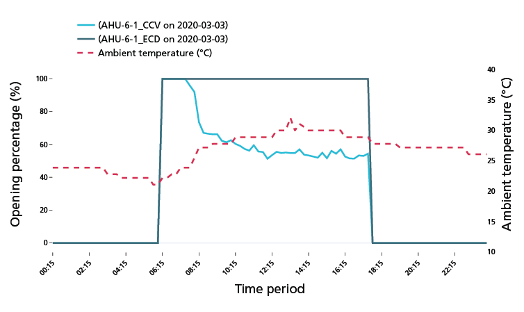
Some faults had less influence on the whole building’s energy performance, but they were identified from the component level anomaly detection (using the approach illustrated in Figure 3). For example, Figure 7(a) shows the economy damper opening level recorded 100 per cent for the entire day, but on the target day, the economy damper was not used at all. This change was substantial; therefore, the AHU was identified as an anomaly by the target deviation analysis. By looking at the economy damper control logic, the root cause analysis finds the economy damper was fully open despite the ambient temperature being quite warm. This is displayed in Figure 7(b). The BMS technician later confirmed that the outdoor air damper was overridden to 100 per cent during the mechanical maintenance and had not been reverted afterwards.
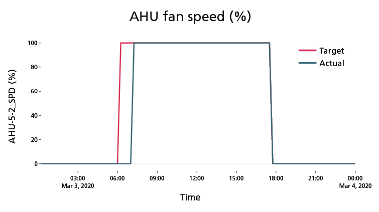
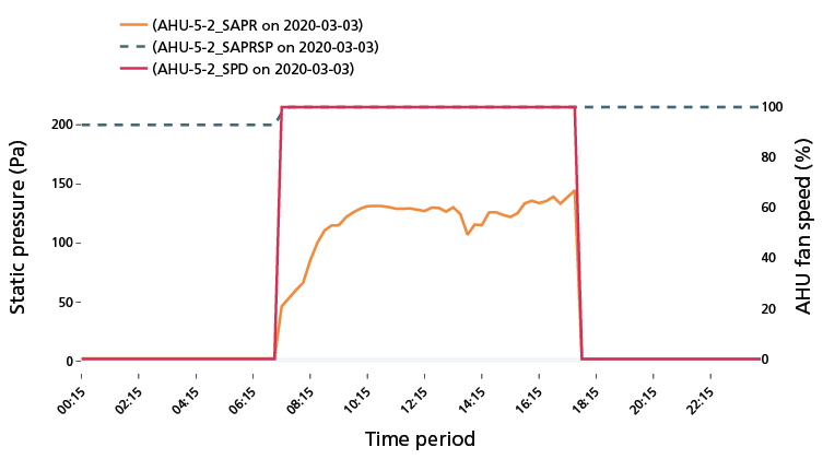
Figure 8(a) shows that, on both subject and target days, the supply air fan of AHU 5-2 was running at the same speed. Interestingly, the target deviation analysis did not manage to identify the fault because the issue also occurred on the target day, but a pre-defined rule captured it. The root cause analysis in Figure 8(b) shows that actual supply air pressure was consistently below the supply air pressure set-point (215Pa) even though the supply air fan was running at full speed. This example highlights the importance of having a “faultfree” model when applying a statistical approach to conducting anomaly detection.
Introduction
Modern commercial buildings are becoming more complicated as the number of sensors, actuators and control loops increases. The building management system (BMS) used to control these components will often generate equipment faults and anomalous behaviour, which causes energy waste, thermal discomfort, and drives up maintenance costs. Such system failures may last for a long time before a facility manager or technician notices them. This necessitates the use of automated fault detection and diagnostics (AFDD) tools to detect operational faults and identify their root causes to ensure fault-free operation.
Commercially available analytical software tools typically use a rule-based fault detection and diagnosis (FDD) approach. Rule-based methods are often specific to certain equipment or systems, and their associated control logic. Without proper configurations and continual refinement of the rule sets, a rule-based FDD tool is likely to produce an excessive number of alerts, many of which are related to detected faults trigged by fine-grained rules, but these faults may have an insignificant impact at a building level. The false alerts would also cause the facility manager or maintenance technician to become fatigued and disengaged1.
As buildings become more data-intensive, analytics based on statistical approaches developed for identifying faults and optimisation opportunities has become an active topic within the building energy research community. Statistical FDD methods look at the systems’ measured inputs and outputs and flag faults if differences are statistically significant or exceed a threshold. Statistical approaches have been applied to detect faults for HVAC components such as variable air volume (VAV) boxes2, air handling units (AHUs) 3 and chiller systems4.
They have also been applied to detect faults at a whole-building level 5. Despite all the research effort, no field studies that use data-driven approaches for whole-building fault detection have been reported in the literature.
In this study, we present a novel model-based anomaly detection method based on a statistical approach. The objective is to identify materially significant system anomalies that impact the whole-building energy consumption. At the whole-building level, we apply a random forest (RF) regressor model to map correlation between weather, occupancy level, calendar effects and interval metering data. The model predicts the expected energy usage by using the independent input variables, and then passes it to a search engine to find “best performance on comparable days” (target days) and uses it as a benchmark to detect anomalies at the building level. At the sub-system level, we use the BMS data and technical specification to build sub-models to estimate the energy consumed by each key HVAC component. If a building’s energy use exceeds the target consumption by an amount considered to be statistically significant, the system will navigate down through the hierarchy and find the most probable solutions to close the gap. The outputs of the algorithm include most significant anomalies to be investigated and their corresponding root cause analysis. The proposed method has been field-tested across 10 office buildings, with significant savings achieved during the period of the trial.
METHODOLOGY
Structure of model-based anomaly detection
AFDD can be approached by either a bottom-up method or top‑down method 6, 7. In the bottom-up approach, performance states of HVAC subsystems, such as zone temperature, pressure, flow, etc., are investigated to detect issues and propagate their effects on building performance. The disadvantage of this approach is that it may pick up issues that are not important for energy efficiency.
Conversely, in the top-down approach, the detection and diagnostics start with flagging energy increases by the building and subsystems (e.g., electricity consumption, cooling/heating systems), which are measured indirectly by monitoring the amount of electricity or gas provided to the building (or subsystem). The top-down approach is selected if the goal is to achieve energy efficiency.
We apply a top-down diagnostic process in this study. The structure of the proposed model-based anomaly detection is illustrated in Figure 1. The workflow is described below. For a given day (actual day) that we wish to find anomalies for, we:
- Build a machine learning model that uses weather and interval metering data to find the “best performing comparable day” (target day) over a given historical window.
- Compare the actual day’s interval meter data to the target day to identify anomalies that affect whole-building consumption (for example, energy spikes, higher baseload, and significant daily energy increase).
- Use BMS data and technical specifications of equipment to estimate the energy usage of individual HVAC components (referred to as “soft meters” in this paper).
- Rank the key energy components: Component usage ranking (for example, soft meter chiller total, soft meter AHUs total) based on the difference between actual day and identified target day.
- Rank anomalies at the sub-component level (for example, AHU‑1, Chilled water pump-2) based on the difference between the actual day and comparable day.
- Discover root causes (e.g., economy damper not used) that explain the system anomaly.

Figure 1. Structure of model-based anomaly detection procedure.
Detecting building level anomaly based on target
When performing building energy modelling, it is assumed that a building’s energy performance characteristics do not change during the training period, and weather inputs can be used as independent variables. However, for buildings that are continually being fine-tuned, the energy performance may improve, leading to the possibility that models trained off historical data may over-predict demand. Similarly, a model could under-predict a building’s energy performance if a building’s performance is trending negatively due to the existence of system faults.
To solve this problem, we built an algorithm to identify “target performance” of the building for any given day and use it as the benchmark for anomaly detection. A detailed description of a statistical approach to generate the target is presented in For building operators, what difference does a target make? by A.C. Roussac and H. Huang8. The target performance represents the best performance a building has achieved for a given period under similar weather and occupancy conditions. In our previous study 9, we found that an RF regressor provides the best balance between accuracy and computational speed when used for building energy modelling. Therefore, the RF has been used to search for the target performance in this study. An outline of the algorithm is as follows:
- Obtain historical data with 15 minutes interval from the database and prepare in a format that can be used for training.
- Remove outlier days, weekends and public holidays from the training set.
- Split the data into training and test sets and feed the inputoutput data into the random forest regression for model training.
- Apply cross validation to find the most optimised combination of hyperparameters, e.g., number of trees in the forest, to avoid overfitting.
- Obtain daily prediction within the training period and store them in the database.
- Apply iterative rules to find comparable days that are similar to the day of interest in terms of weather conditions and daily prediction.
- Once the algorithm finds a pool of comparable days with similar weather conditions and model predictions, the algorithm stops searching.
- From the pool of comparable days, find the days that use the minimum amount of energy.
The above algorithm is designed to find the day in the building’s performance history where the minimum amount of energy was used compared to other days with similar weather conditions, i.e., the day that had the best performance under comparable weather conditions. Figure 2 illustrates how the target profile works. The graph shows that our algorithm has picked up three comparable days, but only “Comparable day 3” was selected as the “target day” because it consumed the least energy among the three comparable days.

Figure 2. Comparison of actual, comparable day and target days’ consumption profile.
Simplified energy model for HVAC components
Once an anomaly is detected at the building level, the next step is to find which sub-component contributes most to the energy increase. To achieve this, we build soft meter models, based on the first law of thermodynamics to estimate energy consumption of individual HVAC components.
Chiller model
Chillers are the most important components in an HVAC system in warm climates, not only because the chiller is the most energyintensive HVAC component, but also because it has complicated dynamics. Accurate modelling of chiller consumption requires technical details and extensive good‑quality BMS data points. The chiller energy model can be simply expressed as:

The chiller power consumption can then be estimated as:


Fan model
Fan power can be approximated as a second-order polynomial function of the total supply air mass flow rate driven by the fan, and the supply air mass flow rate by the fan determined by summation of airflow to each room. This can be expressed as:

Pump model
When estimating the energy usage of the pumps, it is assumed that the enthalpy change of water through the pumps is constant. It is also assumed that the pump volumetric water flow, the pump speed, and pressure difference generated by the pump satisfy the following equations:

Under the above assumptions, the pump consumption can be calculated using the following equation:

Detecting anomalies at the component level
To estimate the savings potential attributable to each component, we demonstrate two statistical approaches in this study: target deviation analysis and peer group analysis. With the target analysis approach, the targeted expected energy usage of individual components is identified and compared to the actual usage. The deviation is calculated using:

Once the deviation is determined, thresholds can be applied for detecting different levels of anomalies. For sub-components, a wider uncertainty buffer zone of 10% is applied to account for the errors generated by soft meter modelling:

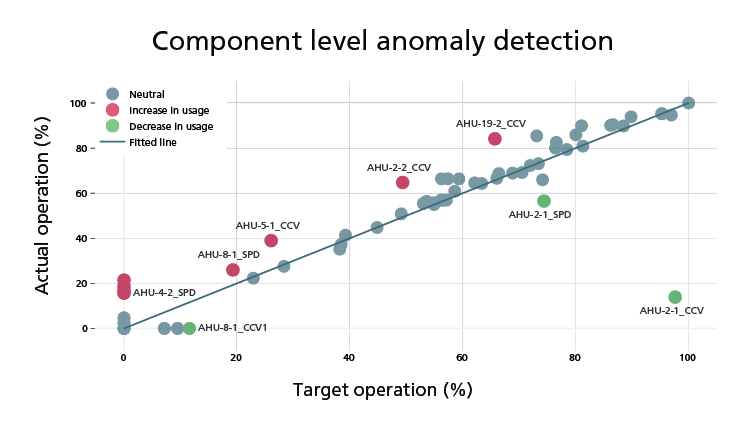
Figure 3 illustrates anomaly detection results by applying the target deviation approach to all the AHU sub-components in an HVAC system. The sub-components include the variables such as cooling valve opening level (AHU_CCV), AHU fan speed (AHU_SPD), and cooling tower fan speed (CT_SPD). Each dot represents the change of usage between actual day and target day. In this graph, the red dots indicate “increase in usage”, the blue dots indicate “neutral”, and the green dots indicate “decrease in usage”. From this graph we can see AHU- 19-2_CCV, AHU‑2‑2_ CCV, and AHU-5-1_CCV are the most anomalous components because they have the largest increase. The straight fitted line illustrates the components that meet the target operation.

Figure 3. Apply the target deviation to pick up anomaly components.
Detecting anomalies at the component level
To estimate the savings potential attributable to each component, we demonstrate two statistical approaches in this study: target deviation analysis and peer group analysis. With the target analysis approach, the targeted expected energy usage of individual components is identified and compared to the actual usage. The deviation is calculated using:
| Component name | Identified anomalies | Action items |
| Chillers 1 and 3 | Inefficient chiller staging control. | Increased chiller staging delay time from 5 mins to 20 mins |
| AHU 13-1 and AHU 5-2 | AHU fan was running at 100% all the time | Removed vague terminal box out of cooling calculation. |
| AHU-6 | Economy damper was used when OA was too warm | Found the outdoor air damper was overridden to 100% open. |
| AHU-4 | 4 Unnecessary operation | Altered the operational schedules. |

Figure 4. Anomalies detected at whole-building level. The actual illustrates electricity profile on March 3, 2020, the target illustrates a best comparable day’s electricity profile, and base range illustrates the range of predicted electricity profile during a baseline period.
Figure 4 compares the actual electricity profile with the target electricity profile at a whole-building level. It shows that the actual usage on the subject day was ~7 per cent higher than the target consumption. The algorithm identified that the most anomalous period of the day happened from 7am to 9am. We can observe a spiky usage from the actual meter readings during this time, while on the target day, the energy usage in the morning looked much smoother.
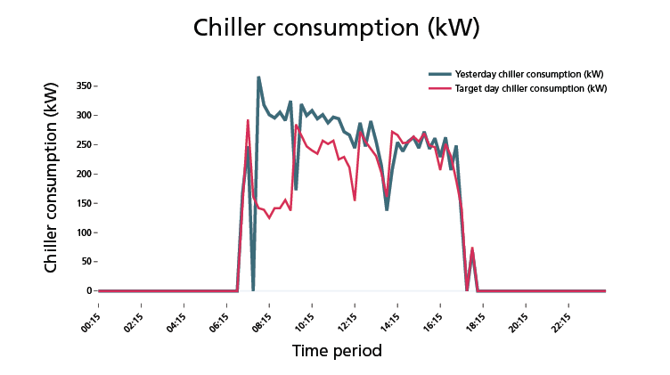
A comparison of chiller consumption is illustrated in Figure 5(a). It clearly shows that the chillers were running harder from 7am to 9am on the subject day compared to the target day, which explains the energy spike that occurred at the whole-building level. Figure 5(b) displays the operational status of different chillers on the investigated day.
After comparing the actual day’s chiller staging with the target, we found that both chillers 2 and 3 were running from 7am to 9am on the investigated day, while on the target day, it was only chiller 1 running. This was later confirmed to be caused by an inefficient chiller staging control strategy. The chiller staging control was then optimised by prolonging the chiller staging delay time and increasing the minimum chilled water temperature set-point.


Figure 5. Comparison of actual and target profile. Top: (a) total chiller consumption (kW), Bottom: (b) actual chiller usage breakdown (kW)


Figure 6. Comparison of actual and target profile. Top: (a) chilled water pump (kW), Bottom: (b) CT fans consumption (kW).
Further, from Figure 6 (a) and (b), we can see chilled water pump and cooling tower fan profiles also show morning spikes, which are tied up to the chiller staging issue.
Some faults had less influence on the whole building’s energy performance, but they were identified from the component level anomaly detection (using the approach illustrated in Figure 3). For example, Figure 7(a) shows the economy damper opening level recorded 100 per cent for the entire day, but on the target day, the economy damper was not used at all. This change was substantial; therefore, the AHU was identified as an anomaly by the target deviation analysis. By looking at the economy damper control logic, the root cause analysis finds the economy damper was fully open despite the ambient temperature being quite warm. This is displayed in Figure 7(b). The BMS technician later confirmed that the outdoor air damper was overridden to 100 per cent during the mechanical maintenance and had not been reverted afterwards.
Figure 8(a) shows that, on both subject and target days, the supply air fan of AHU 5-2 was running at the same speed. Interestingly, the target deviation analysis did not manage to identify the fault because the issue also occurred on the target day, but a pre-defined rule captured it. The root cause analysis in Figure 8(b) shows that actual supply air pressure was consistently below the supply air pressure set-point (215Pa) even though the supply air fan was running at full speed. This example highlights the importance of having a “faultfree” model when applying a statistical approach to conducting anomaly detection.


Figure 7. Top: (a) Comparison of actual and target economy damper operation, Bottom: (b) root cause analysis shows economy damper was open when ambient temperature was high.


Top: (a) Comparison of actual and target AHU fan speed, Bottom: (b) A rule-based algorithm shows the static pressure set-point was not met even when the fan was running at 100%.
Conclusion
We have demonstrated that the proposed model-based anomaly detection method can be effectively used to identify system anomalies that impact whole-building energy consumption. It also provides a root cause analysis and identifies promising solutions, which help managers and technicians to achieve their buildings’ “best-ever” energy performance consistently. Because the anomaly detection method belongs in the “top‑down approach” category, it always prioritises the faults that materially impact energy performance.
Our observation that it generates fewer false alarms would seem to be a significant advantage because building managers and technicians are able to focus attention on a smaller number of issues. Also, because the anomalies are detected based on historical performance data, the solutions often appear quite straightforward. Since the method relies on statistical data analysis, there is always a risk that false negatives will be generated when “healthy” training data are not available. Our future work focuses on the development of an unsupervised learning approach for anomaly detection at buildings that have limited historical data availability.
References
- Dibowski, H., J. Vass, O. Holub, and J. Roj ček.; “Automatic Setup of Fault Detection Algorithms in Building and Home Automation.” In 2016 IEEE 21st International Conference on Emerging Technologies and Factory Automation (ETFA), 1–6 (2016)
- Narayanaswamy, B, Bharathan B, Rajesh G, and Yuvraj A.; “Data Driven Investigation of Faults in HVAC Systems with Model, Cluster and Compare (MCC).” In Proceedings of the 1st ACM Conference on Embedded Systems for Energy‑Efficient Buildings, 50–59. BuildSys ’14. New York, NY, USA: Association for Computing Machinery (2014)
- Zhu, Y, Jin X, and Du Z.; “Fault Diagnosis for Sensors in Air Handling Unit Based on Neural Network Pre-Processed by Wavelet and Fractal.” Energy and Buildings, 44 (January): 7–16 (2012)
- Yan, K, Shen W, Mulumba T, and Afshin A.; “ARX Model Based Fault Detection and Diagnosis for Chillers Using Support Vector Machines.” Energy and Buildings, 81 (October): 287–95 (2014)
- Frank, S, Michael H, Xin J, Joseph R, Howard C, Ryan E, and Gregor H.; “Hybrid Model-Based and Data-Driven Fault Detection and Diagnostics for Commercial Buildings.” National Renewable Energy Lab. (NREL), Golden, CO (United States). https://www.osti.gov/biblio/1290794 (2016)
- House, JM., and Kelly, G.E.; “An Overview of Building Diagnostics.” Diagnostics for Commercial Buildings: Research to Practice (1999)
- Bruton, Ken, Paul Raftery, Barry Kennedy, Marcus M. Keane, and D. T. J. O’Sullivan.; “Review of Automated Fault Detection and Diagnostic Tools in Air Handling Units.” Energy Efficiency 7(2): 335–51 (2014)
- Roussac, A.C. & H. Huang.; For building operators, what difference does a target make? Energy Efficiency, 13(3), 459-471 (2020)
- Huang H and Roussac, A.C.; Predicting peak energy demand in commercial buildings under extreme conditions: by how much can we improve accuracy. CA: ACEEE Summer Study on Energy Efficiency in Buildings (2018)