Feasibility study of wastewater energy transfer for an existing campus building cluster

ABSTRACT

The HVAC-related energy usage of a group of three existing buildings on a Canadian university campus (the “Cluster”) was simulated. Two scenarios were compared: (1) an ambient loop paired with conventional HVAC equipment (boiler plant and cooling tower), and (2) an ambient loop using wastewater energy transfer (“WET”). The study aimed to assess the feasibility of implementing WET as a heating and cooling method for cold-climate institutional buildings, as well as to measure the effects of WET implementation on energy usage, greenhouse gas emissions, and energy costs. It was found that WET implementation provided the Cluster with significant energy savings (23.1% reduction in energy usage) and carbon emissions reductions(70.2% reduction in GHG emissions). Although the WET system had slightly (8.9%) higher energy costs than the conventional system based on 2019 energy pricing, the gap in energy costs between the two systems narrowed significantly (to 0.3%) under projected 2030 energy pricing. As Canadian carbon prices rise in the coming years, it is likely that the financial viability of WET systems relative to conventional HVAC equipment will continue to increase.

introduction

The system investigated in this paper incorporates an ambient loop system and wastewater energy transfer (“WET”) technology.In an ambient loop system, a heat‑transfer medium (often water or a water/glycol mixture) is circulated between/within buildings at ambient or near‑ambient temperatures, typically in the 8–25°C or 15–25°C range.[1] [2] End users upgrade the energy from the ambient loop locally via water‑to‑water heat pumps to produce heating or cooling at‑site.

Ambient loops can be implemented within buildings or building complexes, or on a larger scale as part of municipal energy‑sharing schemes. When employed in this latter capacity, ambient loops represent an advance on older district heating systems, which have traditionally used a supply temperature of 70°C and a return temperature of 40°C.[1] Advantages of ambient loop systems as compared to traditional district heating and cooling systems (as well as traditional communal heating networks) include: the ability to provide simultaneous heating and cooling; the potential to utilize low‑temperature waste heat from various sources (e.g., wastewater, industry, transportation networks, data centres); lowered transmission thermal losses; and a potential reduction in the urban heat island effect.[1] [2] Challenges associated with large‑scale ambient loop networks include increased control complexity and difficulties related to seasonal load balancing.[3] Although at least forty (40) district ambient loops currently operate in European cities,[4]the technology remains an emerging research area. Increased international interest in decarbonisation will likely attract more attention to the possibilities of ambient loop systems in the coming years.

For installations with onsite renewables or buildings utilizing an electrical grid that is not reliant on GHG‑intensive energy sources, wastewater energy transfer (“WET”) presents a sustainable alternative to conventional space cooling and space and water heating. In the wastewater energy transfer process, wastewater‑to ‑water heat exchangers are paired with heat pumps to produce hot and chilled water streams for space heating and cooling. Because temperatures in urban sewers remain relatively constant year‑round, sewers can be used as a heat sink in summer and as a heat source in winter.[5] [6]

WET technology is not yet in common use in North America, but it has been studied experimentally and deployed in a number of buildings worldwide. Large‑scale WET installations such as the Rechts der Isar Medical Centre in Munich and the Okanagan College Wastewater Heat Recovery System prove that WET can be implemented in urban and rural areas with minimal disruption to wastewater flows and infrastructure.[7] [8] Studies indicate that there is substantial unutilised energy potential in urban sewersheds. For example, a 2009 study from Vancouver, British Columbia suggested that an area with a population of 100,000 could produce 300,000GJ of recoverable heat per year, enough to heat 3,000–5,000 single‑family homes.[9]

Further, it is estimated that the potential for recovery of thermal energy from wastewater is much higher than the potential for recovery of chemical energy from wastewater (roughly 90% as compared to 10%), despite the greater scholarly interest that chemical energy in wastewater has raditionally attracted.[10] Wastewater‑source heat pumps are capable of efficiently exploiting these vast resources, having been found to achieve coefficients of performance (“COPs”) of 1.77 to 10.63 in heating mode and 2.23 to 5.35 in cooling mode.[11] Put differently, wastewater‑source heat pumps generally meet the ANSI/ASHRAE minimum standards for water‑source heat pumps, which mandate a COP of 4.3 in heating mode and 3.6 in cooling mode.[12]

Campus building cluster

The cluster of buildings under consideration consists of the Library (“LIB”), Podium (“POD”), and Jorgenson Hall (“JOR”), three interconnected structures on the Toronto Metropolitan University (formerly Ryerson University) campus in downtown Toronto, Canada. The three buildings share a 1970s brutalist style and its associated thermal characteristics (i.e., relatively poor insulation compared to more recent buildings).

The Library, which opened in 1974, stands 10 stories tall.[13]Floors five through 10 contain book storage and private and semi‑private study spaces. The 2nd, 3rd, and 4th floors house computer labs and additional study areas. The Toronto Metropolitan University Archives are located on the 4th floor. Laboratory and archive areas of the building require special cooling and dehumidification.

The Podium is a five‑storey structure connecting the Library in the south with Jorgenson Hall in the north. It contains offices, classrooms, and study spaces. Under normal (non‑pandemic) operations, the lower floors also house a cafeteria‑style food‑service location, as well as banking, open areas for eating and studying, and student services.

Jorgenson Hall, originally constructed in 1971, is a 14‑storey, 58m tower that primarily contains faculty offices and boardrooms. Its design is somewhat unusual, with some rooms having been deliberately designed without windows.[14]

Campus Energy Demand Model

Energy demand for the LIB‑POD‑JOR Cluster was modelled in a powerful analysis program.* Energy modelling was not within the scope of this project; rather, a pre‑existing campus energy model produced by Fung et al. [15] was used to generate seasonal building loads. ASHRAE simulation weather data was used during load modelling.

System configuration 

Heating, cooling, and ventilation in the LIB-POD-JOR Cluster are provided by a water-to-air system, which includes both variable air volume (“VAV”) and constant air volume (“CAV”) systems. The Library and Podium use VAV systems, while Jorgenson Hall uses a CAV/reheat system. 

The LIB-POD-JOR Cluster has a conditioned floor area of just over 37,000 m2 divided into a total of 284 zones. One AHU in the Library (SF-10, 2nd and 3rd floors) and two in the Podium (SF-6, ground and 1st floors; SF-7, 2nd-4th floors) include steam humidification. Simulated per-person ventilation rates range from 18.3-31.2 m3/hr. 

Load estimation for Library-Podium-Jorgenson Hall Cluster  

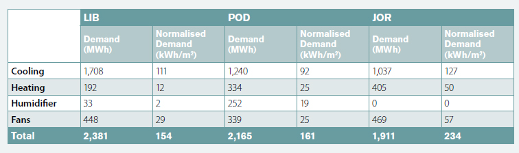
The LIB-POD-JOR Cluster is strongly cooling-dominated due to the large size of the component buildings and the need to compensate for internal heat gains (IHGs) produced by electronic equipment (e.g., computers and lighting). HVAC-related energy demands (cooling, heating, and humidification loads, as well as fan electrical consumption) are shown in Table 1 below. 

Despite their different floor areas and patterns of space usage, the Library, the Podium, and Jorgenson Hall have roughly similar annual HVAC energy demand, with the Library being responsible for the largest portion of the Cluster’s demand at 37% (2,381MWh/year), followed by the Podium at 33% (2,165MWh/year) and Jorgenson Hall at 30% (1,911MWh/year). The Library and Podium have comparable annual HVAC-related energy intensities of 154kWh/m2 and 161kWh/m2, respectively, while Jorgenson Hall is somewhat more energy-intensive at 234 kWh/m2. 

AMBIENT LOOP MODEL

An ambient loop model for the Cluster was developed in a spreadsheet program for two scenarios:

1. ambient loop with conventional heating and heat rejection equipment (boilers and cooling tower), and

2. ambient loop incorporating wastewater energy transfer.

For each scenario, system configuration, modelling methodology, and results (including estimated energy, cost, and GHG emissions) are presented.

MODEL DEVELOPMENT

Hourly building loads – including heating, cooling, and humidification loads – were exported from the model into a comma‑separated values (“CSV”) file. Peak loads, simultaneous loads, and no‑load hours were determined and quantified. A boiler model and an open‑loop cooling tower model were created. Plugins were used to determine the thermodynamic properties of steam/water and moist air, respectively, under given conditions.[16] [17] The boiler and cooling tower models were integrated into a conventional system model, with heat pumps being used to upgrade the available heating/cooling. A fixed ambient loop flowrate was assumed.

Next, a sewer energy profile was constructed based on monitored sewer data from various locations in the Greater Toronto Area. The aim of this sewer energy profile was to approximate the flowrate and seasonal/diurnal temperature variation of the sewers near Toronto Metropolitan University in order to accurately estimate the available wastewater energy for WET. A WET system model was constructed based on the projected sewer energy profile.

Finally, energy usage, GHG emissions, and energy costs were compared for the conventional system and WET system. Emissions factors were derived from the Canadian Ministry of the Environment and Climate Change’s NIR (“National Inventory Report”), while energy costs were taken from Toronto Metropolitan (Ryerson) University’s 2021 Carbon Reduction Roadmap.[18] [19]

CONVENTIONAL SYSTEM

The conventional system model consists of:

1. a cooling tower model,

2. a boiler model, and

3. a heat pump model, integrated with a fixed‑flowrate ambient loop.

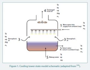
An open‑circuit cooling tower was modelled as per the schematic in Figure 1 below. Temperature (T, in °C) and specific enthalpy (h, in kJ/kg•K) are given at each state point, along with the relative humidity (RH, unitless) and humidity ratio (ω, unitless) of the incoming and outgoing air.

The specific enthalpy of air is denoted ha (in kJ/kg•K), while the specific enthalpy of saturated liquid water and saturated water vapour are denoted hf and hg, respectively (also in kJ/kg•K).

Because the flowrate of the ambient loop is constant, warm water entering the tower from the ambient loop (State 1) and cooled water returning to the ambient loop (State 2) share a single flowrate, m ̇ w (in kg/s). Likewise, air enters and exits the tower at the same mass flowrate, m ̇ a (in kg/s). The tower is assumed to run when there is a net demand for cooling. Analysis was performed using the spreadsheet plugin to determine water/steam properties and the Excel Psych plugin to determine the properties of moist air.

Ambient loop flowrate (m ̇ w) was set to a constant value of 100 kg/s, with makeup water rate and airflow rate determined on an hourly basis as a function of ambient loop flowrate and the properties of supply (State 1) and return (State 2) water in the ambient loop. (The selected ambient loop flowrate is further justified below.)

State points were fixed as follows:

1. State 1: The thermodynamic properties of the supply water from the ambient loop are determined by the amount of heat rejected by the heat pumps in the LIB‑POD‑JOR Cluster.

That is:

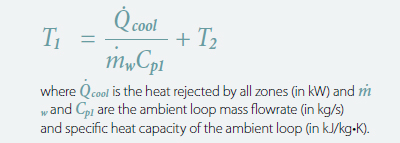
2. State 2: Water at State 2 is at the ambient loop temperature, which, when there is net demand for cooling, is defined as being 5°C above the outdoor wet‑bulb temperature.

That is:

When there is no net demand for cooling, ambient loop temperature is constant at 15°C.

3. State 3: State 3 is outdoor ambient air. Dry‑bulb and wet‑bulb temperatures provided by CarrierHAP were used to establish the state.

4. State 4: State 4 is moist leaving air. The following assumptions were made to determine the properties of leaving air at State 4:

a. Temperature at State 4 was taken as the average of outdoor ambient temperature and supply temperature from the ambient loop.

That is:

b. Relative humidity at State 4 was assumed to be 20% higher than outdoor relative humidity, up to a maximum of 100%. That is:

5. State 5: Makeup water, which compensates for evaporation, is also treated as being at the same temperature as the ambient loop temperature.With these relationships in place, the mass flowrate of air through the cooling tower was found through Equation 1:

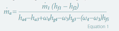
Note that when the system is in heating mode hf1 = hf2and therefore the mass flowrate of air is 0 and the cooling tower is off/bypassed.

Equation 2 below gives the mass flowrate of makeup water in kg/s:

As with airflow through the cooling tower, the makeup water rate is 0 when cooling is not required.

Boiler efficiency was set to a constant value of 75% following the work of Kwiatek.[6] The boiler and cooling tower models were integrated to create a conventional system ambient loop model capable of meeting the complete heating, cooling, and humidification demands of the LIB‑POD‑JOR Cluster.

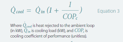
Once loads were extracted from the model, heat extracted from and rejected to the ambient loop were defined as follows:

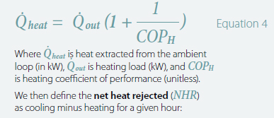
We then define the net heat rejected (NHR) as cooling minus heating for a given hour:

NHR determines how much cooling must be provided by the cooling towers or (if negative) how much heating must be supplied by the boilers. Boiler energy use and chiller fan rate and makeup water rate were set to ensure that NHR was always met.

Heat pump COP in cooling mode (COPc) was determined based on condenser water temperature (T2 = TAL) from a curve in the work of Kwiatek, and ranged between 5.4 and 6.[6] Heat pump COP in heating mode (COPH) was set to 4.2, the high end of the normal range for water‑source heat pumps in heating mode as per Natural Resources Canada.[21] Note that this is a simplification, as COPH would not remain static in actual operation.

We define a further parameter, ΔTHP, representing the temperature difference in degrees Celsius between the indoor setpoint (20°C for heating and 22°C for cooling) and the ambient loop temperature. This difference remains low throughout the year, as the ambient loop temperature is constrained between 8.8°C and 29.9°C due to:

1. a constant ambient loop temperature of 15°C being used during heating season, and

2. the limited variation of outdoor air temperature outside of heating season.

In the special case in which TAL < 22°C – that is, the ambient loop temperature is already below the cooling setpoint – then the system enters free cooling mode. In free cooling mode, a bypass is employed and the heat pumps are not required to operate.

Ambient loop flowrate was set to 100kg/s of water (via a trial‑and‑error process) in order to:

1. ensure sufficient available energy, and

2. minimise the temperature difference between supply and return streams of the cooling tower (ΔTCT, in °C). ΔTCT reaches a maximum of 8.72°C in the model, a value which is well within the normal range for a commercial cooling tower.

WET SYSTEM

For the WET system, a wetwell – a structure that receives sewage for handling – will be constructed to tap into one of the sewers adjacent to the university campus. Wastewater will be screened for debris, passed through a bank of shell‑and‑tube wastewater‑to‑water heat exchangers housed in an Energy Transfer Station (“ETS”), and – once its energy has been extracted – returned to the sewer. The shell side of the heat exchanger will be wastewater, while the tube side will be clean (ambient loop) water. This system configuration will ensure that only clean water circulates on the university side of the heat exchanger. The fluid pressure will also be higher on the tube side of the heat exchanger to ensure that in the event of a rupture clean water enters the wastewater side, and not vice versa, though it should be noted that such an emergency is unlikely.

Although the WET system is capable of meeting the Cluster’s complete heating and cooling needs, a boiler plant and/or cooling tower(s) for may be retained for redundancy depending on local legislation and the preferences of the building operators. Regulations regarding redundancy may differ depending on the exact configuration of the WET system.

SEWER TEMPERATURE AND FLOWRATE ESTIMATION

Sewer temperature and flow data were received from Toronto Water for several sites in the Greater Toronto Area. In order to estimate available wastewater energy in a manner consistent with the outdoor air temperatures generated in the analysis model (and because temperature data was available only for the August–October 2018 period), it was necessary to determine a correlation accounting for the relationship between sewer temperature and:

1. outdoor dry‑bulb temperature, and

2. time of day.

Sewer temperature fluctuates seasonally with outdoor air temperature, with average sewer temperatures being higher in summer and lower in winter. Additionally, sewer temperature varies predictably within a 1–2°C window throughout the day; temperatures are lowest around 7am–8am and rise steadily towards a high point in the late morning/early afternoon (11am–2pm).

Temperatures then drop steadily until they reach another low point around 5pm–6pm, before climbing towards their highest point around midnight. Although there is considerable day‑to‑day variation in the exact shape of the sewer temperature curve, this general pattern of two peaks and two valleys holds true throughout the year.

The flows from Sewer MH101, Site 005 were used to generate a correlation between wastewater temperature, seasonal outdoor dry‑bulb temperature, and time of day according to the following method:

■A fifth‑degree polynomial trendline was generated to represent variation in wastewater temperature as a function of time of day (“Correlation A”).

■Mean daily ambient temperature and mean daily wastewater temperature were correlated using a line of best fit (“Correlation B”).

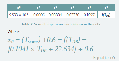
■To capture the effect of seasonal variation, the x0 value of the fifth‑degree polynomial (y‑intercept) was replaced with the estimated mean daily wastewater temperature as determined from Correlation B.

■An offset of +0.6°C was applied to reduce error.

RMSE between estimated sewer temperature and recorded sewer temperature under this method (“Correlation C”) was 0.73. The maximum modelled wastewater temperature was 25.6°C, while minimum modelled wastewater temperature was 19.6°C, values consistent with most urban sewersheds.[22] [23] The coefficients of the line of best fit used are shown in Table 2 below.

The estimated temperature profile was paired with a full year of actual flow data from a different monitoring site (103–119) to generate a complete temperature/flowrate profile.

WET SYSTEM MODELLING

Maximum available sewer energy (i.e., energy available if the entire sewer flow is utilised) was calculated according to Equation 7 below:

Where m ̇ is the mass flowrate of the sewer, cp is the specific heat capacity of water (wastewater), and ΔT is the inlet‑outlet temperature difference across the wastewater side of the heat exchanger, here taken to be 3°C due to municipal safety limits on wastewater temperature.

A 5°C difference between water and wastewater streams was assumed – that is, ambient loop temperature was taken to be 5°C higher than the sewer temperature in the cooling season and 5°C lower than the sewer temperature in the heating season. When these limits were imposed (assuming the same heat pump configuration and efficiencies as in the conventional system), the peak heat rejected to the ambient loop (peak cooling) was 3,647kW, while the peak heat extracted from the ambient loop (peak heating) was 702kW. Meanwhile, the lowest available sewer energy at any point during the year is 5,416kW (occurring in late March). Thus, even if the energy of the sewer is only partially utilised, the WET system will not struggle to meet the peak demands of the LIB‑POD‑JOR Cluster.

COMPARISON WITH CONVENTIONAL SYSTEM

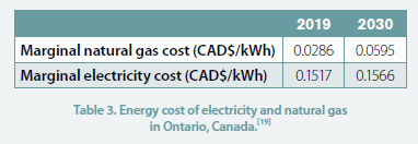
Marginal energy costs in 2019 and 2030 are shown in Table 3 below. Energy costs are from Toronto Metropolitan (Ryerson) University’s 2021 Carbon Reduction Roadmap. Natural gas costs are predicted to rise significantly due to carbon prices gradually increasing throughout the decade, though it should be noted that all energy cost predictions are highly speculative, and that natural gas pricing in particular is volatile and heavily market‑reliant.

GHG emissions factors are shown in Table 4. All emissions factors are from the Canadian Ministry of the Environment and Climate Change’s National Inventory Report. For electricity‑related emissions, the average emissions factor (“AEF”) is used; the AEF represents the most basic quantification of carbon emissions, and does not take time‑based shifts in the grid’s energy mix (or other complexities of electricity generation) into account.

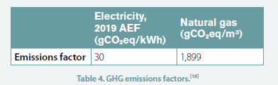
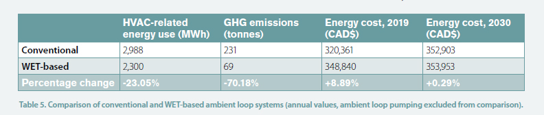
Table 3 below shows the annual energy usage, GHG emissions, and energy costs of the conventional and WET‑based ambient loop systems. While the WET system provides a significant (70.18%) reduction in GHG emissions and a moderate (23.05%) reduction in HVAC‑related energy use, annual energy costs are slightly (8.89%) increased under 2019 energy pricing. However, when 2030 energy pricing is applied, the annual energy costs of the WET system only marginally (0.29%) exceed those of the conventional system. This suggests that rising carbon prices in coming years are likely to make WET a more and more financially viable alternative.

conclusion

The simulation shows that WET is a feasible solution for the Cluster, providing meaningful reductions in annual energy use and GHG emissions, with only a slight (based on 2019 energy pricing) or marginal (based on 2030 energy pricing) increase in annual energy costs. These results suggest that WET may find productive applications within cold‑climate institutional buildings more generally. Future refinements to the Library‑Podium‑Jorgenson Hall WET model will include: a complete financial analysis including return on investment (“ROI”) calculations, the addition of a detailed ambient‑loop pumping model, and the development of a hybridised WET‑conventional model (i.e., a model in which WET and conventional HVAC equipment are used alternatingly or simultaneously throughout the year) with optimisations for energy usage, cost, and GHG emissions. It is hoped that the present study will provide a basis for future WET‑related research.

Acknowledgements

This research was supported by funding from Toronto Metropolitan University, Mitacs Accelerate, and Noventa Energy Partners.

References

[1] London Energy Transformation Initiative, LETI Climate Emergency Design Guide: How New Buildings Can Meet UK Climate Change Targets.

[2] A. Revesz, P. Jones, C. Dunham, G. Davies, C. Marques, R. Matabuena, J. Scott and G. Maidment, “Developing novel 5th generation district energy networks,” Energy, vol. 201, 2020.

[3] S. Buffa, A. Soppelsa, M. Pipiciello, G. Henze and R. Fedrizzi, “Fifth-Generation District Heating and Cooling Substations: Demand Response with Artificial Neural Network-Based Model Predictive Control,” Energies, vol. 13, 2020.

[4] S. Buffa, M. Cozzini, M. D’Antoni, M. Baratieri and R. Fedrizzi, “5th generation district heating and cooling systems: A review of existing cases in Europe,” Renewable and Sustainable Energy Reviews, vol. 104, 2019.

[5] Y. Gu, T. Wang, W. Liu and F. Ma, “Energy-saving Analysis and Heat Transfer Performance of Wastewater Source Heat Pump,” Applied Mechanics and Materials, vol. 694, pp. 211-217, 2014.

[6] C. Kwiatek, Techno-Economic Feasibility of Wastewater Energy Transfer (WET) Systems for Cold Climates (Master’s Thesis), Toronto, Ontario, 2020.

[7] Huber, “Wastewater heat utilisation and reuse of process heat at Munich university hospital “Klinikum rechts der Isar”,” [Online]. Available: https://www.huber.de/huber-report/ablage-berichte/energy-from-wastewater/wastewater-heat-utilisation-and-reuse-of-process-heat-at-munich-university-hospital-klinikum-rechts-der-isar.html. [Accessed 29th April 2022].

[8] British Columbia Ministry of Community & Rural Development, “Integrated Resource Recovery Case Study: Okanagan College Wastewater Heat Recovery,” [Online]. Available: https://www.waterbucket.ca/gi/sites/wbcgi/documents/media/270.pdf. [Accessed 29th April 2022].

[9] C. Johnston, E. Lindquist, J. Hart and M. Homenuke, “Four steps to recovering heat energy from wastewater,” British Columbia Water & Waste Association Watermark, Craig Kelman & Associates, vol. 18, no. 2, pp. 16-18, 2009.

[10] X. Hao, J. Li, M. C. M. van Loosdrecht, H. Jiang and R. Liu, “Energy recovery from wastewater: Heat over organics,” Water Research, vol. 161, pp. 74-77, 2019.

[11] A. Hepbasli, E. Biyik, O. Ekren, H. Gunerhan and M. Araz, “A key review of wastewater source heat pump (WWSHP) systems,” Energy Conversion and Management, vol. 88, pp. 700-722, 2014.

[12] ASHRAE, “Standard 90.1-2019, Energy Standard for Buildings Except Low-Rise Residential Buildings,” 2019. [Online]. Available: https://ashrae.iwrapper.com/ASHRAE_PREVIEW_ONLY_STANDARDS/STD_90.1_2019. [Accessed 29th April 2022].

[13] M. Lefebvre, “The Library, the City, and Infinite Possibilities: Ryerson University’s Student Learning Centre Project,” 2013. [Online]. Available: http://library.ifla.org/id/eprint/62/1/081-lefebvre-en.pdf. [Accessed 15 October 2021].

[14] Architectural Conservancy Ontario, “Ryerson University; Jorgenson Hall,” [Online]. Available: https://www.acotoronto.ca/show_building.php?BuildingID=1758. [Accessed 15 October 2021].

[15] A. S. Fung, M. Z. Rahman, H. Taherian, M. M. Selim and M. Hossain, “Energy Audit and Base Case Simulation of Ryerson University Buildings,” ASHRAE Transactions, vol. 121, 2015.

[16] University of Alabama, “Excel Stuff,” [Online]. Available: https://www.me.ua.edu/me215/f07.woodbury/ExcelStuff.html.

[17] UC Davis Western Cooling Efficiency Center, “Psych: An Open Source Psychrometric Plug-in for Microsoft Excel by Kevin Brown,” [Online]. Available: https://wcec.ucdavis.edu/resources/software-resource-applications/.

[18] Ministry of Environment and Climate Change Canada, National Inventory Report 1990-2019: Greenhouse Gas Sources and Sinks in Canada, 2021.

[19] Ryerson University Climate and Energy Working Group, Carbon Reduction Roadmap — Draft Framework, Toronto, Ontario, 2021.

[20] M. J. Moran, H. N. Shapiro, D. D. Boettner and M. B. Bailey, Fundamentals of Engineering Thermodynamics, 8th ed., Hoboken, NJ: John Wiley & Sons, 2014.

[21] Natural Resources Canada, “Heating and Cooling With a Heat Pump,” 2022. [Online]. Available: https://www.nrcan.gc.ca/energy-efficiency/energy-star-canada/about/energy-star-announcements/publications/heating-and-cooling-heat-pump/6817. [Accessed 2022].

[22] H. Xiaodi, J. Li, M. C. M. van Loosdrecht, H. Jiang and R. Liu, “Energy recovery from wastewater: Heat over organics,” Water Research, vol. 161, pp. 74-77, 2019.

[23] S. S. Cipolla and M. Maglionico, “Heat recovery from urban wastewater: analysis of the variability of flow rate and temperature in the sewer of Bologna, Italy,” Energy Procedia, vol. 45, pp. 288-297, 2014.

About the author

Monica Brands is the sustainability coordinator for Noventa Energy Partners, a renewable energy company based in Toronto, Ontario. Brands is also a Masters student whose work focuses on novel heat pumps, building energy efficiency, and wastewater energy transfer. She has studied aerospace engineering at Queen Mary, University of London, and mechanical engineering at Toronto Metropolitan University in Ontario, Canada. She has co-authored three papers on heat pump technology and one on the impact of ventilation on airborne virus transmission.