Augmented heat recovery for transcritical CO2 refrigeration systems 

Samantha Bothma M.AIRAH, BEng Mechanical, ARPEng 

Abstract 

There is an incentive to improve energy efficiency, reduce equipment footprint and save costs on refrigeration systems in supermarkets. Heat recovery of vapour-compression refrigeration systems is a method to achieve all three of these requirements. Traditionally, refrigeration systems are designed to cool by transferring heat away from the source (or food) and expelling it to the atmosphere. Instead of expelling it to the atmosphere, this energy can be used for other purposes. The amount of heat that can be recovered depends on the system operation. Various techniques can be used to harness all the available heat in a system, as well as adjusting the system to augment additional heat. Carbon dioxide (CO₂) proves to be an ideal refrigerant for this, with the additional benefit of being a natural refrigerant with high operating temperatures.  

Introduction 

The benefit of CO₂ (R744) as a refrigerant is that it is a safe, natural refrigerant with an ozone depletion potential (ODP) of 0 and a global warming potential (GWP) of 1. It is also non-toxic and non-flammable. Since CO₂ has a critical point of 31.1°C, the system will often run in supercritical operation if required, where it has independent temperatures and pressures above this point. This results in a high potential for heat recovery in this region due to the higher operating pressures (> 90 bar) and high discharge temperatures (> 100°C). As a result, heat recovery may be augmented from these CO₂ systems. 

CO₂ also has a high volumetric efficiency, which means that less is needed to achieve the same heat transfer. This also means components are smaller for CO₂ refrigeration systems. In supermarket refrigeration systems operating on CO₂ (specifically transcritical systems or systems that operate above and below the critical point), waste heat that would otherwise be transferred to the atmosphere through a gas cooler or condenser can be recovered and used for other purposes such as space heating, domestic water heating, underfloor heating or evaporator coil defrost. CO₂ is also readily available and inexpensive, making it an excellent choice for refrigeration systems. 

1. Heat recovery potential 

Heat recovery potential is dependent on the system operation as well as the heat exchanger design itself. The design of the heat exchanger plays a pivotal role in the actual heat recovered from the system. 

1.1 System design 

Heat recovery potential is dependent on the refrigerant properties as well as the ambient conditions. Specifically for space heating, and for valid heat recovery, compressor discharge temperatures need to be higher than the heating hot water (HWH) temperatures. Heat recovery potential is based on the change in enthalpy across a component multiplied by the mass flow of the refrigerant. A higher temperature and pressure generally result in a higher enthalpy. 

The table below shows a comparison in the calculations for three different refrigerants based on the assumed standard conditions outlined below. 

Outdoor ambient temperature: 10°C 

Saturated suction temperature (SST): -10°C 

Superheat (SH): 5K 

Condensing temperature (SCT): 18°C for CO₂ and 30 for other refrigerants 

Pressure drop across heat exchangers is zero 

Isentropic compressor efficiency: 0.7 defined by the equation below and Figure 1. 

$$\begin{array}{c}{𝜂}_C=\frac{W_s}{W_{real}}=\frac{h_{2s}-h_1}{h_2-h_1} \#\left(1\right)\end{array}$$

Where: 

η_C: isentropic compressor efficiency 

W_s: isentropic compressor work 

W_real: real compressor work 

h_2s: specific enthalpy of the gas at the discharge of the compressor for isentropic process 

h₂: specific enthalpy of the gas at the discharge of the compressor for real process 

h₁: specific enthalpy of the gas at the suction of the compressor 

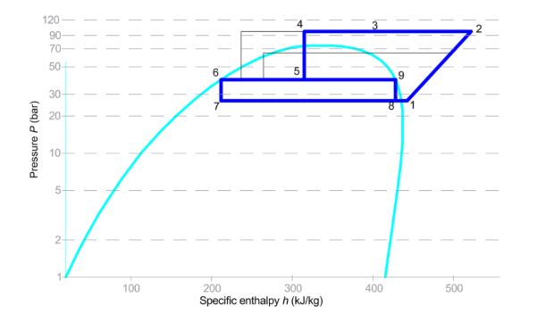
Figure 1: Refrigeration vapour compression process diagram and P-h diagram 

Figure 2: Pressure-enthalpy diagrams for R404a, R134a and R744 superimposed on one another 

Figure 2 above indicates points 1–5 on the R744 process diagram corresponding to Figure 1. The same points apply to the R32, R134a and R404a process diagrams. The conditions at point 2 are determined from the isentropic efficiency as defined in equation 1. The differences in enthalpy change across the three different refrigerants for the same conditions are clear and align with the results found in Table 1. The properties in Table 1 are derived from P-h diagrams ​(TLK Energy, 2025)​ and from a property calculator ​(Coolprop, 2025)​, and the enthalpy at the outlet of the heat exchanger is the enthalpy at 100% saturation conditions at condensing pressure. The condensing temperature is specific to the refrigerant and typical for winter conditions. 

Table 1: Summary of enthalpy calculations for various refrigerants 

*x is defined as the quality or the vapour fraction of the fluid under saturation conditions 

COPheating=QHeatingWC=(h2−hHX)(h2−h1) #(2)$$\begin{array}{c}{COP}_{heating}=\frac{Q_{Heating}}{W_C}=\frac{{(h}_2-h_{HX})}{{(h}_2-h_1)} \#\left(2\right)\end{array}$$

R744 (CO₂) has a much better COP for heat recovery potential at the same conditions as synthetic refrigerants, and thus it is widely accepted that transcritical CO₂ systems would be designed and installed with heat recovery. Even when operating in subcritical mode (condensing, not gas cooling), the potential for heat recovery is significant.  

1.2 Heat exchanger design 

To calculate the heat transfer of a heat exchanger, the (LMTD) logarithmic mean temperature difference (LMTD) method can be used. Using high temperature discharge gas from compressors allows for a high LMTD. A high LMTD represents a high ratio of heat transfer to heat exchanger surface area. LMTD can be calculated for different configurations of heat exchangers. Counter-current heat exchangers allow for higher outlet temperatures of the cold fluid and lower outlet temperatures of the hot fluid. The relationship between the temperatures along the length of the heat exchanger is shown in Figure 3, adapted from Cengel & Ghajar (Cengel, 2011) and Bitzer (Bitzer Software, 2025). 

Q=U×A×LMTD #(3)$$\begin{array}{c}Q=U\times A\times LMTD \#\left(3\right)\end{array}$$

Where:  

Q is the amount of heat transferred (W) 

U is the heat transfer coefficient (W/km²) 

A is the surface area of the heat exchanger (m²) 

LMTD is defined below (for counter current heat exchangers)  

LMTD=ΔTA−ΔTBln(ΔTAΔTB) #(4)$$\begin{array}{c}LMTD=\frac{{∆T}_A-{∆T}_B}{ln\left(\frac{{∆T}_A}{{∆T}_B}\right)} \#\left(4\right)\end{array}$$

Where: 

ΔTA=Thot,in−Tcold,out #(5)$$\begin{array}{c}{∆T}_A=T_{hot,in}-T_{cold,out} \#\left(5\right)\end{array}$$

ΔTB=Thot,out−Tcold,in #(6)$$\begin{array}{c}{∆T}_B=T_{hot,out}-T_{cold,in} \#\left(6\right)\end{array}$$

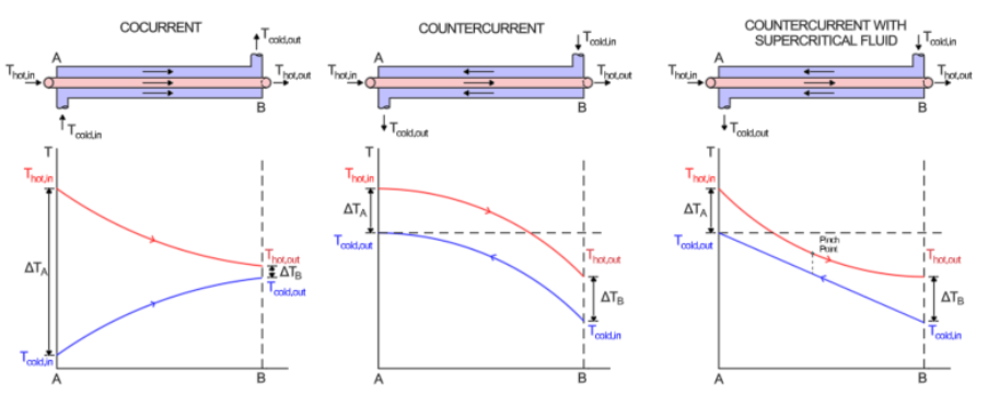
Figure 3: LMTD of cocurrent and counter-current heat exchangers 

The pinch point of a heat exchanger refers to the closest approach temperature between the hot and cold fluid. The temperature difference between the hot and cold streams should not be lower than the minimum approach temperature (MAT) ​(Ting Liang, 2022)​ as indicated in Figure 4 below. 

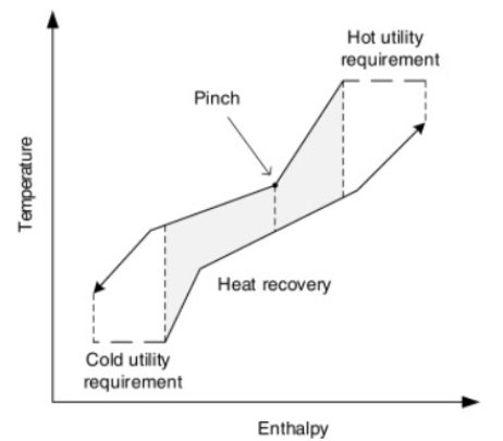
Figure 4: Composite curves of hot and cold streams in heat exchangers ​(Peng, 2018)​ 

2. Stages of heat recovery 

The amount of heat recoverable on a refrigeration rack is dependent on operating conditions, including discharge pressure and temperature, as well as the mass flow rate. Typically, refrigeration systems do not operate at total design capacity. The following stages of heat recovery allow for different discharge conditions (pressure and temperature). 

2.1 Stage 1: Passive heat recovery 

Passive heat recovery occurs when the transcritical CO₂ system is operating as normal, typically in subcritical mode where the discharge gas is condensing due to the ambient conditions for which heating would be required. The discharge gas from the MT and HT suction groups is diverted to the heat reclaim heat exchanger. The heat from the discharge CO₂ gas is transferred to the water, usually entering at 25°C.  

2.2 Stage 2: Active heat generation  

Additional heat is generated by gradually increasing the discharge pressure to a maximum predefined heat reclaim gas cooler set point (typically a pressure of 90–95 bar). The refrigeration system is now operating in transcritical mode. The PC compressors would not engage unless the MT capacity is at 100%.  

2.3 Stage 3: Active heat generation with increased flash gas production 

The maximum discharge pressure is maintained while the gas cooler outlet temperature is increased from the design approach to ambient (typically 2K) to the maximum allowable gas-cooler outlet temperature (typically 38–40°C). This temperature is determined by the relationship between gas cooler pressure and gas cooler leaving temperature for optimal COP. For example, at 92 bar, GCLT would be 38°C ​(Liao, 1998)​. Increasing the flash gas production results in additional mass flow through the MT compressors.  

2.4 Stage 4: Active heat generation with engagement of heat pump evaporators 

To induce further heat generation, additional load may be required on the MT or HT suction. This is obtained with the engagement of heat pump evaporators (also referred to as false load or outdoor evaporators). These heat pump evaporators are designed to meet the space heating conditions. Since the rack is assumed to be operating below maximum capacity, the now spare capacity on the MT or HT suction can be used to manage the heat pump evaporators. Theoretically, the operating points of stage 4 are the same as stage 3, however, there is increased mass flow and thus increased heat recovery. 

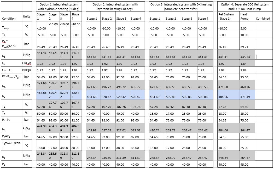
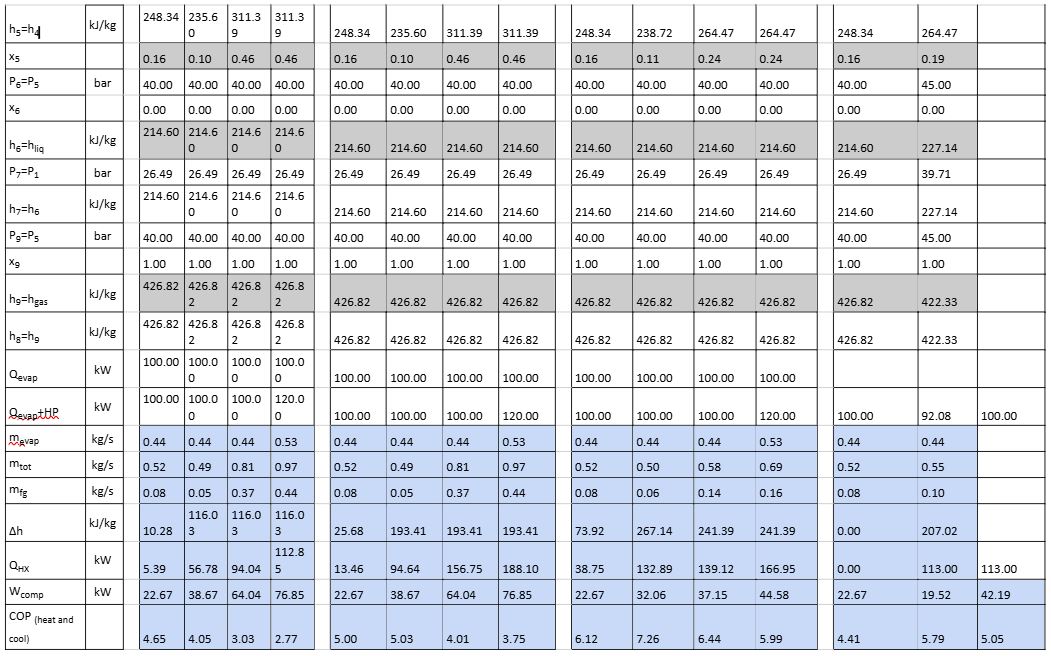
2.5 Stages of heat recovery: Example  

Below is a summary of first principal calculations used to determine the heat recovery potential for the various phases explained above. It is based on the original conditions as stipulated in Figure 3, unless otherwise stated. It is important to note that this example only considers an MT load and there are no parallel compressors; as such, the flash gas is compressed by the MT compressors. Also, the MT load is set at 100 kW (no part load is considered). The COP is calculated for cooling and heating mode and is defined by equation 7. The subsequent results in Table 2 are based on the following assumptions: 

MT capacity: 100kW @ -10°C SST 

OAT: 15°C 

Condenser KTD: 10K 

Approach temperature in transcritical: 2K 

Isentropic compressor efficiency: 0.7  

HX CO₂ outlet temperature: 50°C 

Water inlet temperature: 25°C 

Water outlet temperature: 50°C 

Minimum pinch point allowed: 2K 

Heat pump evaporator capacity: 20kW (additional evaporation load with a total load of 120kW) 

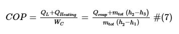
Where: 

Q_L: Evaporation capacity (kW) 

W_C: Compressor work (kW) 

h_x: enthalpy at points defined in figures 5–7 

m_tot: total mass flow (kg/s) 

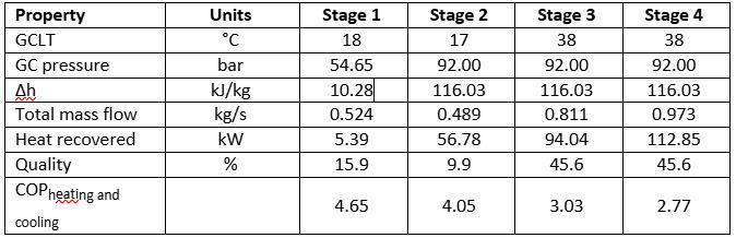
 Table 2: Calculation results for stages 1–4 of heat recovery 

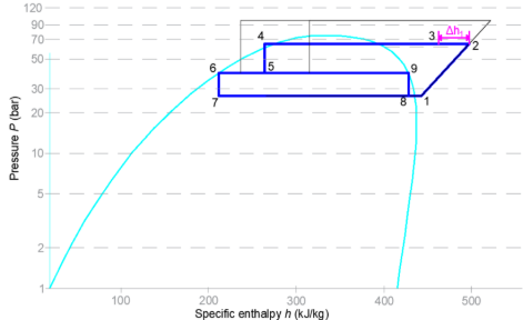
Figure 5: Stage 1 heat recovery 

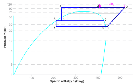
Figure 6: Stage 2 heat recovery 

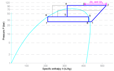
Figure 7: Stage 3 and 4 heat recovery 

There is a COP penalty when augmenting heat, as the COP of a CO₂ system when operating in transcritical mode is lower than when it is operating in subcritical mode (i.e., condensing), but it is still an improvement over electric duct heaters or an electric boiler.  

2.6 Comparison between hydronic heat recovery, direct heat recovery and separate heat pump system 

There are various options for heat recovery from a refrigeration system: hydronic heating and direct heating. Another option for space heating would be a standalone CO₂ heat pump to supply the heating capacity required.  

The following assumptions apply: 

• Hydronic heating with 50°C CO₂ outlet temperature as per the example in section 2.5 

• Hydronic heating with 40°C CO₂ outlet temperature (all other conditions the same as the example in section 2.5) 

• Refrigeration system with direct heating assumes a 25°C GCLT ​(Alemu, 2025)​, with all possible heat recovered, and an operating pressure of 75 bar 

• Standalone refrigeration system operating in stage 1 conditions as per the example in section 2.5, as well as a CO₂ heat pump operating at the same heating conditions as direct heating, but with an evaporation temperature of 5°C. 

When adding 20kW of heat pump evaporators to the options and designing the heat pump to align with the example in section 2.5, the following is achievable in stage 4 heating: 

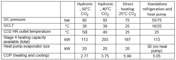
Table 3: Comparison of different heating methodologies 

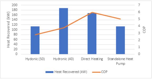
Figure 8: Comparison of different heating methodologies 

Comparing the options above, a lower CO₂ outlet temperature results in a better COP, as well as significantly more heat recovery. Direct heating offers the best COP, however, not as much heat is recovered compared to a hydronic system with a lower CO₂ outlet temperature due to the operating conditions. A standalone heat pump offers a good COP but requires additional equipment and is more cost prohibitive.  

Potential risks, including CO₂ leaks in the AHU, thermal fatigue and oil management need to also be considered when deciding on direct heating for heat recovery. The benefit of direct heating is that it offers an exceptionally efficient means of heating at lower operating pressures than that required for hydronic heat recovery, as well as a reduction in the equipment required (such as a water tank, pumps etc.).  

3. Theoretical versus realistic heat recovery 

Although GCLT in stage 3 (active heat generation with increased flash gas production) calls for a maximum GCLT of 38°C, this may need to be reduced to prevent the gas cooler fans from hunting in low ambient temperatures. Options to manage fan hunting include, but are not limited to, splitting the gas cooler coil, splitting the gas cooler fans (during stage 3, a maximum of half the fans are active), or limiting the GCLT to a more achievable setpoint.  

During low ambient temperatures, store load may operate even lower than the design point, which would lead to lower actual refrigeration connected loads and thus less heat recovery is available. Consideration for a portion of the refrigeration loads during the design phase will ensure adequate heat recovery. 

Refrigeration fixture diversity factor will also lead to lower actual refrigeration connected loads.  

System design affects the amount of heat recovery augmented by altering discharge temperatures. An example of this would be a PC suction superheater heat exchanger. 

The MT SST determines the KTD of the heat pump evaporator. With a design OAT in mind, the KTD across the coil could vary depending on the MT SST. Consideration needs to be given to maintain sufficient superheat to prevent liquid flood back and ensure stable EEV operation.  

Although a design point for the CO₂ outlet temperature is selected for the heat exchanger in theory, the actual CO₂ outlet temperature could be higher or lower. This would result in additional heat transfer to the water and thus better heat recovery from the system as per Figure 9. The gas cooler could need to remove less heat from the system and thus could lead to hunting. This difference in temperature should also be considered when performing the LMTD calculations, as a lower outlet temperature of CO₂ would result in less potential heat transfer of the heat exchanger itself, so there is a balancing act in having a higher heat recovery potential and the actual heat transfer possible through the heat exchanger. 

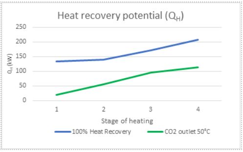
Figure 9: Comparison of heat recovery potential for different conditions 

Low ambient temperatures and high relative humidity could lead to rapid ice build-up on heat pump evaporators. An example of this is that, at an OAT of 3°C and RH of 95% (possible during fog), the dew point Is 2.3°C. This would result in rapid ice-build up on the heat pump evaporator coil, which is why the defrost strategy is of the utmost importance. Consideration must be given to defrost initiation and termination temperatures, as well as the location of the defrost probes. The defrost methodology will also play a role in managing the ice build-up. The potential strategies include off-cycle defrost, hot gas defrost or electric defrost. 

Pinch points need to be considered for heat exchangers. This is the point in the heat exchanger where the cold fluid and hot fluid differ by the smallest difference. By recovering 100% of the heat in the system, your heat exchanger needs to be large. Heat exchanger size and cost need to be considered when determining the design conditions, i.e., amount of heat recovery as a percentage or CO₂ outlet temperature of the heat exchanger, water operating temperatures or system operating conditions. 

Conclusion 

CO₂ offers an opportunity to recover waste heat that would otherwise be transferred to the atmosphere. Given the high operating temperatures and pressures of a transcritical CO₂ system, the benefits are unlike any other commercially suitable refrigerant. With the added benefit of being a natural refrigerant, it is a good way to integrate systems such as space heating and domestic water heating. It is important to design systems correctly to ensure maximum heat transfer, including the heat exchanger and the refrigeration system. Various options exist for heat recovery, including hydronic heating and direct heating depending on user requirements. There are several practical considerations including component performance, defrost strategies and actual system load

Appendix (Tables of calculated conditions/values) 

Table 1 calculations verified by first principles (values highlighted in grey are sourced from click here – values in blue are calculated). 

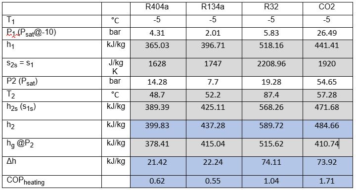
Table 2 and Figure 8 calculations are based on the following formulae and properties in grey are derived from: click here properties in blue are calculated. 

Points 2,3,4 and 5 on the P-h diagram change depending on the stage of heating and operating conditions. 

$$m_{tot}=m_{evap}+m_{flash gas}$$

$$m_{tot}{h}_4=m_{evap}{h}_6+m_{flash gas}{h}_9$$$$x_5=\frac{h_5-h_9}{h_6-h_9}$$$$W_{comp}=m_{tot}\left(h_2-h_1\right)$$$$Q_{evap}=m_{evap}\left(h_1-h_7\right)$$$$Q_{HX}=m_{tot}\left(h_2-h_3\right)$$$$Q_{HX-100\% HR}=m_{tot}\left(h_2-h_4\right)$$

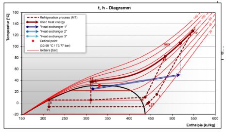
The t-h diagram above shows what is expected for a 25°C water inlet, 50°C water outlet and 38°C CO₂ outlet (worst case for pinch point). The calculated pinch point from the Bitzer Software is 11.7K.

References

Alemu, A. & Hudson, J (2025). Innovative space heating and cooling using an R744 heat pump: A comparative study. Ecolibrium. Retrieved from https://theecolibrium.com/2025/04/02/innovative-space-cooling-and-heating-using-an-r744-heat-pump-a-comparative-study/.
Bitzer Software. (2025). Retrieved from https://www.bitzer.de/websoftware/.
Cengel, Y. A. (2011). Heat and Mass Transfer Fundamentals and Applications, Fourth Edition. In Y. A. Cengel, Heat and Mass Transfer Fundamentals and Applications, Fourth Edition. Singapore: McGraw-Hill.
Coolprop. (2025, 10 30). Coolpropgit. Retrieved from CoolProp: https://coolprop.org/
Hydrofluorocarbon refrigerants – global warming potential values and safety classifications. (2024, December 13). Retrieved from Australian Government Department of Climate Change, Energy, the Environment and Water: https://www.dcceew.gov.au/environment/protection/ozone/rac/global-warming-potential-values-hfc-refrigerants#nonhfc-refrigerants
Liao, S. &. (1998). Optimal heat rejection pressure in transcritical carbon dioxide air conditioning and heat pump systems. Natural Working Fluids.
Peng, X. (2018). Liquid Air Energy Storage: Process Optimization and Performance Enhancement. University of Birmingham: Chemical Engineerin.
Ting Liang, T. Z. (2022). Thermodynamic Analysis of Liquid Air Energy Storage (LAES) System. Encyclopedia of Energy Storage, 232-252.
TLK Energy. (2025). log p-h Diagram. Retrieved from TLK Energy: https://tlk-energy.de/en/phase-diagrams/pressure-enthalpy