Optimisation of Economy Cycle Operation and Supply Air Temperature Control for VAV systems

ABSTRACT

A range of supply air temperature control strategies for a VAV-serviced office building is tested via simulation across three major temperate Australian climate zones. This is used to determine the extent to which the modulation of supply air temperature control affects the effectiveness of economy cycle operation on an annual basis. The results show some worthwhile improvements in economy cycle savings but limited ability to assess a priori whether a given approach will work well. On this basis, at least while fixed annual controls are retained, it is concluded that the primary challenge for economy cycle optimisation is to avoid a poor outcomes rather than finding the perfect optimised control. 

INTRODUCTION

Large commercial buildings in temperate Australia commonly use variable air volume (VAV) air-conditioning systems. This preference is also common in the US but is not universal; the UK and Europe, for instance, strongly prefer fan coil systems. From an energy efficiency perspective, one of the key benefits of any system that uses air as its primary form of heat transport is that it can use an economy cycle. Economy cycle is a process whereby outside air provides “free cooling” in the right conditions. This is achieved by increasing the outside air supply from the statutory minimum (in Australia, 7.5–10 L/s per person, equating to typically around 1 L/s per m2 in a typical office) to full airflow (typically between 2.5–5 L/s per m2 for centre zones and 4–7 L/s per m2 for perimeter zones in a typical office), while rejecting the equivalent volume of relief air from the building.  

The benefits of economy cycle control have been calculated via simulation to be in the region of 8–10% of total HVAC energy use in temperate Australia [Bannister and Zhang, 2014]; correlative studies of empirical performance indicated that the presence of economy cycle correlates with a 0.6-star improvement in NABERS base building ratings [Bannister et al 2009]1. A further benefit, especially salient in the post-COVID era, is the significant increase in ventilation rate that occurs while the economy cycle is in operation. 

Bannister and Zhang (2014) also demonstrated that the savings associated with economy cycle can be significantly eroded by control configurations that unnecessarily limit the times at which the control can operate2. Furthermore, given the mechanical ability of an economy cycle to flood the building with outside air when it is not beneficial, the presence of an economy cycle is not without risk to building performance. 

Previous work by the authors has focussed firstly on economy cycle enablement criteria [Bannister and Zhang 2014] and latterly on supply air temperature control [Bannister and Zhang, 2015]. In this paper, the question of supply air temperature control is examined further, with particular emphasis on the benefits of decoupling the economy cycle and cooling coil for supply air temperature control. 

Purpose of this paper 

This paper aims to test supply air temperature control strategies to optimise the energy savings achieved via economy cycle operation, for variable air volume systems.  

The analysis is based on simple reset controls for supply air temperature as used in industry.  

In the analysis presented below, the conditions of economy cycle enablement are considered to be resolved and are not examined further. 

ECONOMY CYCLE CONTROLS 

In general, the HVAC industry lacks conventions concerning the detail of HVAC control, resulting in a divergence of practices. In Australia, anecdotally, this situation appears to have improved somewhat over the past decade due to the impact of NABERS, which has led to some refinement and convergence in control practices in parts of the office sector at least. Nonetheless, this remains largely undocumented.  

The common structure of most economy cycle controls is: 

1. Economy cycle is enabled when outside conditions are suitable. Typically, the economy cycle is enabled when the outside air is cooler than the return air temperature, with additional considerations for humidity either in the form of a dewpoint lockout or outside air/return air enthalpy comparison to ensure that excessive latent loads are not brought into the building. A dry bulb temperature lockout is often added as a failsafe against the accidental operation of economy cycle in grossly unsuitable conditions. 
2. The economy cycle operates to achieve the supply air setpoint as a first stage of cooling ahead of the cooling coil. This is normally achieved by using a PI/PID loop for the supply air temperature loop in which the first stage of control operates the economy cycle from 0–100%, and the second stage opens the chilled water valve 0–100%. This ensures that the economy cycle is fully utilised before the chilled water is used. 

External references for economy cycle control are relatively rare:  

• AIRAH (2011) published guideline control sequences. The supply air temperature control used a reset schedule that reduces the supply air temperatures from 23°C to 12°C (or system minimum) as the control zone temperature ranges from 21°C to 24°C. 

• ASHRAE Guideline 36 (2018) presents a supply air temperature control that combines a supply air temperature reset from 18°C to system minimum as the outdoor air temperature varies from 16°C to 21°C. It also incorporates a test and respond control to vary the supply air temperature between this reset and the minimum to meet control zone cooling requirements. The guideline notes that tuning of these variables is required on a case-by-case basis. 

The situation is further complicated by the limitations of simulation packages in representing supply air temperature control (without going into more complex programming modes). For the two most used packages in Australia: 

• IES<VE>2021 can undertake supply air temperature control based on resets that provide a fixed relationship between supply air temperature and other variables. This enables it to provide a good representation of many common simple controls. 
• The simulation package3 provides a control method (Setpoint Manager: Warmest) that calculates the supply air temperature that meets the maximum loads on the system at maximum zone flow. 

Notably, neither of these packages can fully represent the control from ASHRAE Guideline 36. Furthermore, the simulation package algorithms are based on the knowledge of the zone loads, which is data unavailable to a real control system. As a result, the Setpoint Manager: Warmest configuration can only be approximated in real building controls. 

The Theoretical Case for Decoupling 

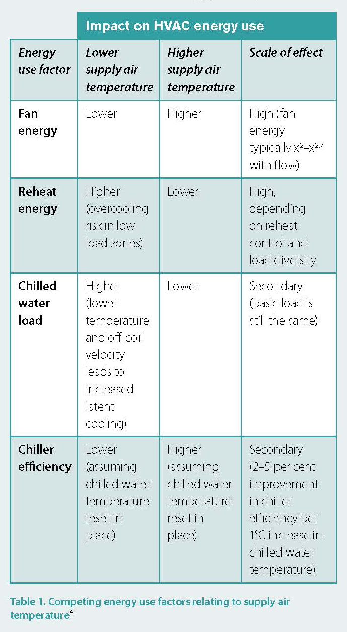
When considering the question of supply temperature control for VAV systems, it is necessary to consider the competing factors at play, as summarised in Table 1. 

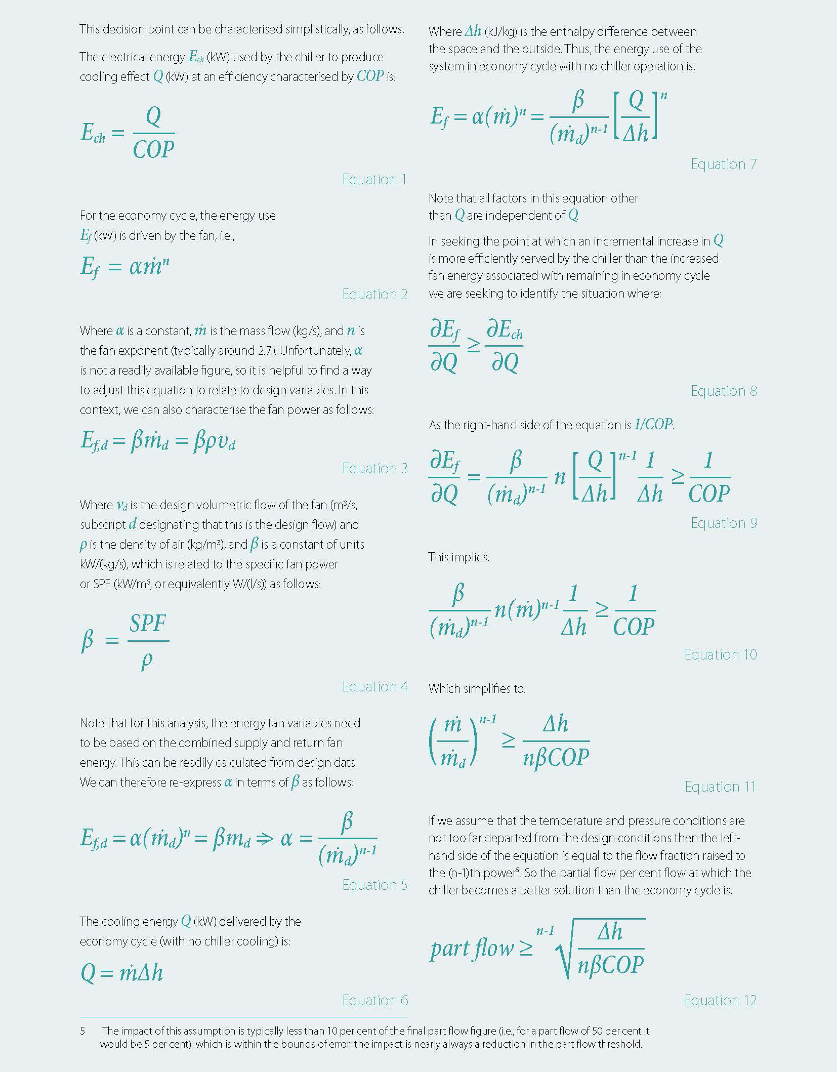
In chiller-only operation (i.e., cooling without economy cycle), the high sensitivity of fan energy to flow leads to the general industry position that low flow/low-temperature operation is preferable. However, in economy operation, the situation is more complex, as there is a decision point that relates to when it is more efficient to use the chiller to reduce the supply air temperature and maintain the current air supply volume than to increase the air volume at fixed supply air temperature.

In practice, this means that there is a percentage flow for a given AHU above, which it is no longer economical to increase airflow. This flow limit: 

• increases when Δh is large, i.e., the outside air is much cooler than the inside air; and conversely 
• decreases as Δh decreases, i.e., the outside air temperature approaches the indoor air temperature.  

Equipment efficiency also plays a predictable role: a more efficient chiller or a less efficient fan system will reduce the part flow limit.  

In practice, the part flow figure turns out to only be below 100% at relatively low values of Δh, as shown in Figure 1. 

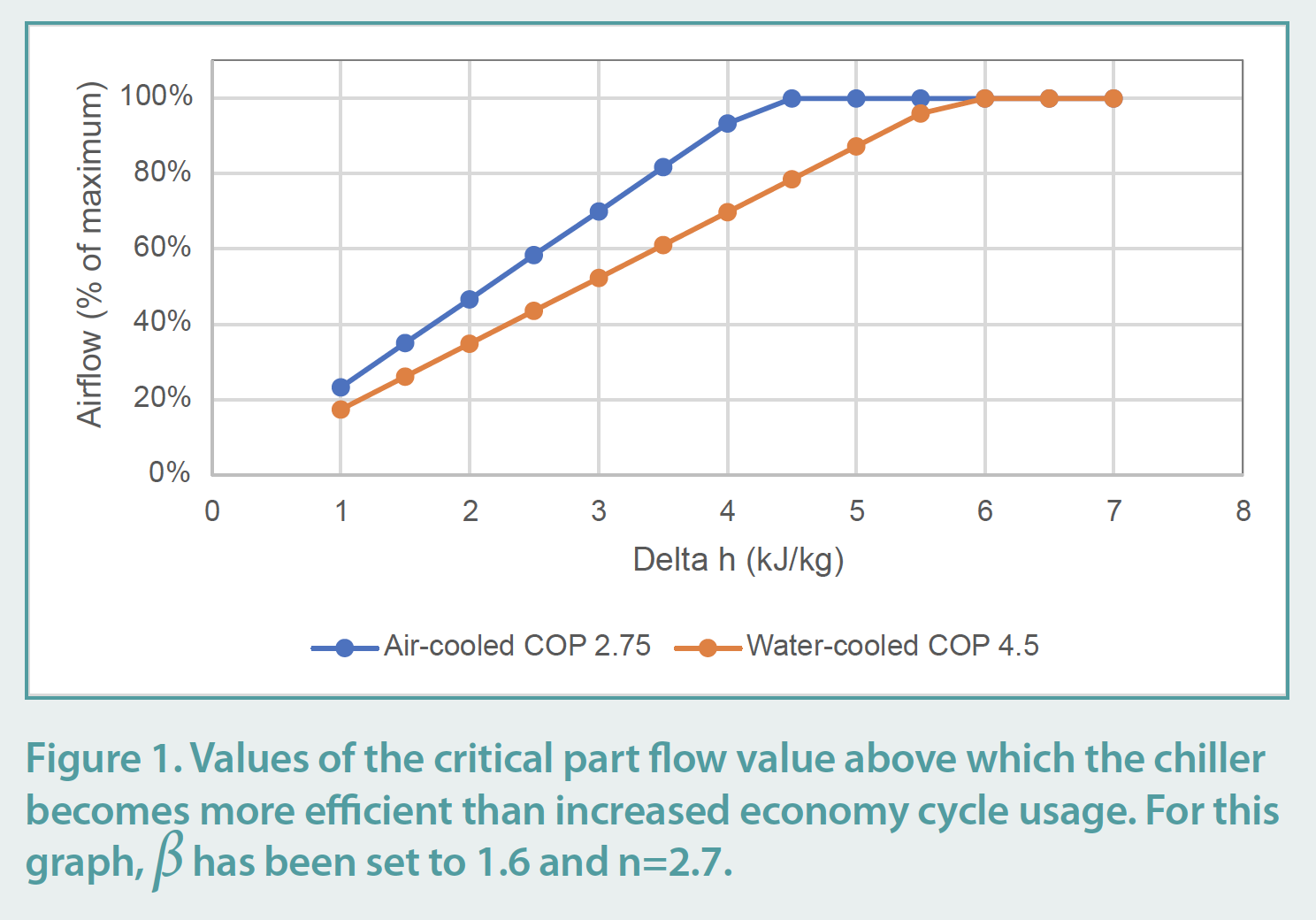
The implication from this is that it is preferable to maintain full economy cycle operation – with no chiller operation, right down to the region of a Δh of 4-6kJ/kg, which is typically around 2-3°C difference between return air and outside air.  

This simplistic analysis does not consider the issues associated with latent cooling. Still, it does provide a priori indication that a high temperature, high flow configuration is potentially beneficial in economy cycle, in contrast to the use of low temperature, low flow in chiller-only operation. This, in turn, implies that there may be a benefit in decoupling the control of supply air temperature (for both the economy cycle and the chilled water coil, separately) from that of the chilled water coil in non-economy cycle operation. However, it does not indicate the scale of that benefit. 

SIMULATION ANALYSIS 

Simulations for this project were conducted in IES<VE>, using the model as outlined in the Appendix to this paper. IES is accredited under ASHRAE140, BESTEST and EN13791 and ISO52000 and, importantly, is well configured to represent supply air temperature controls using reset schedules in a manner very similar to how they are used in real buildings.  

The analysis commenced with an open-ended exploration of the impact of a wide range of supply air temperature schedules and some variants of system configuration on performance, as described in Section 3.1. This was followed by a more specific analysis of candidate supply air temperature resets that appeared to perform best from the exploratory work, as presented in Section 3.2. 

Initial Problem Exploration

An extensive initial exploration of possible supply air temperature effects was conducted to understand the energy impacts of the key control parameters. This exploration included 18 to 21 scenarios per climate zone of different arrangements of supply air temperature control for the economy cycle and chilled water coil control, focussing mainly on adjusting the centre point of the respective resets. Most scenarios used 0.5°C control zone reset ranges, although a set of 2°C reset range scenarios was also included. All scenarios featured the same VAV configuration with a heating proportional band from 21–21.5°C and a cooling proportional band from 23.5–24°C. 

The depth and complexity of the results from this exploration indicate considerable scope for further study and control nuance to be explored, much of which would appear to lie beyond the scope of current industry control practice. For this paper, however, a decision was made to focus on what can be achieved while maintaining simple approaches that reflect current industry practice. In this context, it was found that: 

• Different AHUs serving different thermal characteristics typically (but not uniformly) exhibited the same behaviours concerning energy use relative to various setpoint combinations. This indicates that using a generic control sequence for all AHUs is not incompatible with a reasonable efficiency outcome. A notable exception was when the centre zone AHU was reconfigured to have no reheat (i.e., all heating at the AHU) and average temperature control (as appropriate for AHUs without reheat). This is discussed further below. 
• The position of the economy cycle reset had little influence on cooling-related energy use. This is important as the authors had previously thought that a lower temperature economy cycle reset would provide a worthwhile precooling benefit by operating the building at a lower overall temperature during the availability of economy cycle cooling. Indeed, it was found that such a benefit does exist but is massively outweighed by the increased use of reheat caused by the lower supply air temperature, even in a well-zoned building with limited load diversity. It would be expected that this problem would be exacerbated in a real building with significant diversity in occupancy.  
• The use of average rather than high select control6 reduced the optimum temperature range for the economy cycle reset. This is unsurprising as the average temperature will tend to be lower than the high select temperature. 
• There was a mild energy benefit obtained from operating the cooling coil reset in economy cycle operation so as to prefer higher air volumes and higher supply air temperatures, as suggested by the analysis in Section 2. This is due to the fan energy penalty being less than the chiller energy penalty in meeting the higher loads. For the test building, this corresponded to the cooling coil reset operating between 23.5–24°C, which is the same temperature range as the zone-level VAV cooling proportional band.  

• In periods when economy cycle was not available, it was found preferable to engage the cooling coil at a lower temperature to maintain a low temperature/low flow configuration. For the test building, this generally led to a cooling coil reset in the range 23–23.5°C, which implies minimum temperature operation being achieved before the high-select zone reaches its cooling proportional band. 
• Different climates resulted in different optimum control configurations, although a small set of control configurations tended to perform close to optimally across all three climates. 

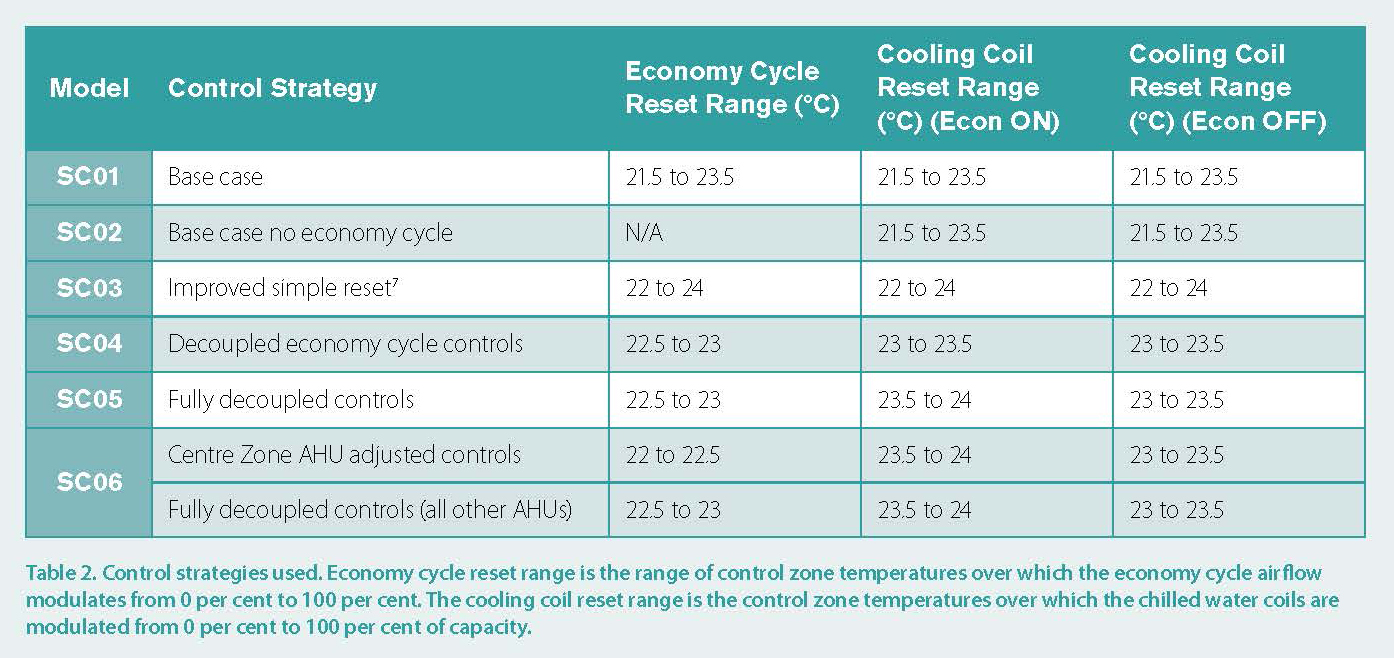
Based on these findings, the control configurations shown in Table 2 were selected to represent the best outcomes. These configurations are constrained to fixed reset schedules that are (largely) constant between air handlers and are unchanged throughout the year. 

Scenario Analysis 

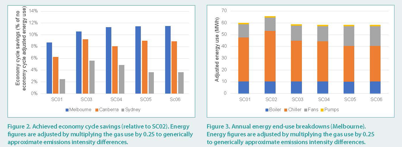
Results for the scenarios in Table 2 are summarised in Figure 2 for the three cities modelled (Sydney, Melbourne and Canberra, representing NCC climate zones 5, 6 and 7, respectively). For presentation, the energy results from the simulations have been modified by multiplying the boiler gas energy by 0.25. This provides a generic adjustment that represents the difference between gas emissions and electricity emissions without introducing the complication of state-by-state differences8.  

Two key results are evident in Figure 2: 

• Optimum scenarios are different from climate to climate.  
• The decoupled control approaches (SC04-06) offer marginal improvements in economy cycle performance in Melbourne and Canberra but perform poorer than the enhanced simple approach in SC03 and underperform the simple scenario in Sydney. 

This indicates that as a minimum, a degree of customisation of supply air setpoint control is required on a city-by-city basis. This would also imply that customisation needs to occur on an individual building basis. 

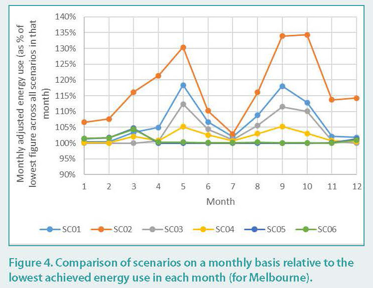
Using Melbourne results as an example, it is possible to see how the chiller and fan energy modulate between scenarios, as shown in Figure 3. 

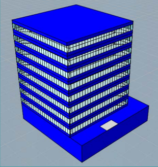
Similarly, using Melbourne as an example, the monthly energy use can be compared between scenarios, as shown in Figure 4. It can be seen from the figure that different scenarios perform better in different months, suggesting that there is some potential for further optimisation using adjustments relating to outdoor conditions. However, the associated benefits are relatively small; for Melbourne, Canberra and Sydney respectively, the sum of the lowest monthly adjusted energy use figures was 1.1%, 1.4% and 0.005% lower than the lowest energy scenario. 

Discussion

The simulation results indicate that while there is a significant difference between a poor economy cycle control and improved control, the various combinations of more complex controls only offer limited improvements. In particular, the decoupled scenarios do not provide improvements relative to well-selected simple coupled control of SC03. This suggests that the additional complexity of a decoupled control may not be merited.  

However, the more challenging finding from the results is that it is not necessarily easy to determine which control configuration will result in a poor or improved outcome without a detailed study. As various exploratory simulations were conducted for this paper, minor differences in HVAC configuration and larger scale adjustments like the use of water-cooled rather than air-cooled chillers appear to change optimum scenarios. As a result, the major conclusion from this study is that the determination of the ideal supply air temperature control for a project is problematic and far from self-evident. This may present a risk for projects, especially if the simulation package cannot readily represent realistic controls. A further consequence of this finding is that the specific optimisations presented in this paper should not be considered generalisable.  

Using a simple fixed annual control configuration, or even one changed on a seasonal monthly basis, may be constraining optimisation factors. In essence, the limited differentiation in the results presented may indicate the common failings of all the tested scenarios (the use of the same control irrespective of AHU or the dynamic operating conditions) rather than physical performance limits. Although the exploratory simulations conducted for this study hinted at opportunities for further optimisation, they also showed that the problem was highly complex and in need of extensive further work before any useful result could be achieved. It remains unclear whether such further optimisation would yield significant further performance improvements. 

Given the results to date, it may be that the main benefit of a more complex and dynamic control approach may not lie in the fine optimisation of performance, but rather the creation of a more robust method to identify an acceptable optimisation customised to the individual circumstances of a given building.  

Conclusion

This paper has explored the impact of supply air temperature control on the effectiveness of economy cycle operation. While theoretical analysis suggests that there may be benefits to decoupling the control of the cooling coil during economy cycle from its control at other times, the simulation studies presented do not show an advantage relative to a well-selected simpler, coupled control that is reflective of current practice. However, the results also highlight the successful selection of such a control is non-trivial and dependent on the details of an individual building’s design.  

It is concluded that the selection of an industry-standard supply air temperature reset that delivers efficient outcomes for a given building is difficult. Indeed, for current simple control approaches, it would appear that a sufficient goal would be to avoid a poor outcome rather than attain an ideal outcome. Achievement of reliably optimised benefits from economy cycle controls across diverse buildings may justify more complex and dynamic control approaches than the simple fixed controls used in this study and current industry practice. 

APPENDIX 1

A typical Australian office building was modelled as the base case for this study. The simulation follows NCC 2019 Section Deemed-to-Satisfy provisions and NABERS Commitment Agreements Handbook for Estimating NABERS Ratings Version 2.0 – September 2021.

APPENDIX 1.1 BASIC BUILDING CHARACTERISTICS

The base model has these characteristics:
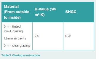
■ 8-storey building with underground carpark
■ 50 per cent WWR
■ NCC 2019 Section J compliant building envelope
■ 25m by 25m floorplate, 4 perimeter and 1 centre
zone per floor, the total area is 5,000m²
■ Floor to ceiling height 2.7m, Plenum height 0.9m
■ HVAC: VAV system with central plant

APPENDIX 1.2 WEATHER FILES

TMY weather files appropriate to the region were used in the simulation. TMY weather files were developed by Department of Industry, Science, Energy and Resources and CSIRO for building energy simulation. The building was modelled in Sydney, Melbourne and Canberra

APPENDIX 1.3 MODELLING SOFTWARE

Modelling was executed in IES which was developed by Integrated Environmental Solutions Limited and has passed ASHRAE 140, BES TEST and CIBSE TM33 accreditation. The program has been widely used in Australia and has widespread international acceptance.

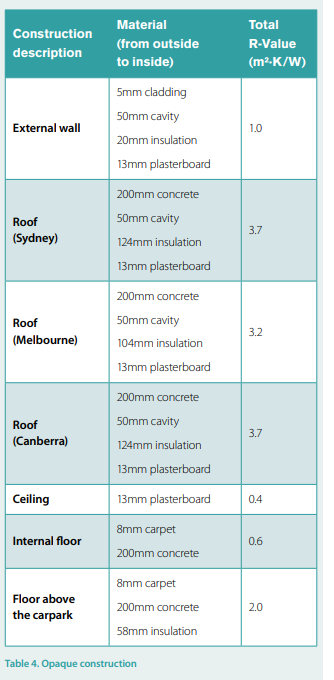
APPENDIX 1.4 BUILDING CONSTRUCTION

Double glazing with the characteristics shown in Table 1 was used in the simulation.

The opaque construction was modelled to achieve NCC 2019 Section J compliant building envelope R-Value:

APPENDIX 1.5 INTERNAL LOADS

The internal loads were modelled as follows:
■ Occupancy: 10m² per person. Sensible heat gain of 75W/person and latent heat gain of 55W/person
■ Equipment: 11W/m²
■ Lighting: 4.5W/m² distributed equally between office space and ceiling plenum.

The operation schedules for occupancy, equipment and lighting were set as per NABERS default schedules.

APPENDIX 1.6 INFILTRATION

Infiltration for the main building was modelled as 0.7 ACH throughout all zones when there is no mechanically supplied outdoor air; and 0.35 ACH at all other times. Infiltration for underground carpark is modelled as 2 ACH for 24/7

APPENDIX 1.7 HVAC

HVAC system was modelled as follows:
■ Zone temperature control. The zone temperature control was to 22.5°C with a dead band from 21.5°C to 23.5°C and 0.5°C proportional band. The VAV box minimum turndown was set to 30 per cent for perimeter zones and 50 per cent for centre zones.
■ AHU configuration. Separate AHUs were provided for each facade and for the centre zone.
● AHU supply air fans were modelled as having an efficiency of 70 per cent, motor efficiency of 90 per cent and an x2.7 turndown (representing variable pressure control). AHU return air fans were modelled as having an efficiency of 70 per cent, motor efficiency of 90 per cent and an x2 turndown (representing fixed pressure control).
● Perimeter AHUs only have cooling coils. The heating was supplied to perimeter zones via hot water terminal reheats.
● Centre AHU has both cooling and heating coils. No terminal reheats were modelled in centre zones.
● All AHUs were configured with a temperature economy cycle with a dewpoint lockout at 14°C and a dry-bulb lockout at 24°C. The AHU cooling supply air temperature setpoint and economy cycle setpoint were reset from 12°C to 24°C based on high-select zone temperature for perimeter zones and average temperature for centre zones.
● The centre AHU heating supply air temperature setpoint was reset from 24°C to 30°C base on average zone temperature.
■ Central plant. The cooling was supplied by two identical air-cooled chillers. The COP and IPLV were modelled as per NCC2019 Section J. The heating was supplied by two identical condensing boilers. The boiler efficiency was modelled as per NCC2019 Section J

Acknowledgements

The support of DeltaQ Pty Ltd and Enerefficiency Pty Ltd in funding this work (in‑kind) is gratefully acknowledged.

References

1. AIRAH, 2011 DA28 Building Management and Control Systems Application Manual. Control sequences are documented in Appendix B.
2. ASHRAE 2018 ASHRAE Guideline 36-2018 High Performance sequences of Operation for HVAC Systems
3. Bannister, P, Salmon, S, Quinn, R, 2009. “What Really Makes Buildings Efficient: Results from the Low Energy High Rise Project” AIRAH Preloved Buildings Conference, Melbourne, 2009.
4. Bannister, P, Zhang, H, 2014. “What simulation can tell us about building tuning” Ecolibrium December 2014
5. Bannister, P, Zhang, H, 2015. “Optimisation of Supply Air Temperature Controls for VAV Systems in Temperate Australia”, Building Simulation 2015, Hyderabad, India, 2015

Top Honours

The lead author of this paper, Dr Paul Bannister, F.AIRAH, was recently awarded

AIRAH’s highest honour – the James Harrison Medal.

To read more about him, scan the QR code. Dr Bannister’s fellow authors were Enerefficiency director Hongsen Zhang; and DeltaQ intern Alisha Garg.