Disaggregation of precipitation data applicable for climate‑aware planning

Abstract
High-temporal-resolution precipitation data of the past along with other data of weather elements are required for applications in the design and simulation of built environments. However, the available data of precipitation is either low-resolution, e.g., daily, or not long enough to produce reliable and climate-responsive results for built environment applications.
In this paper, we develop a stochastic algorithm based on Markov chain Monte Carlo (MCMC) methods to generate hourly temporal resolution precipitation data given daily precipitation data. To improve the accuracy of the generated disaggregated precipitation series, a combination of data recorded for several weather elements such as temperature, relative humidity, wind speed and cloud cover are incorporated along with the precipitation data.
The algorithm uses simulated annealing based on the Metropolis-Hastings algorithm. In this model, desired properties, such as the correlation between the generated precipitation series with other weather elements, are formulated in an objective function through which the algorithm generates the desired precipitation series.
Finally, we conduct a comparison between these two algorithms. The outputs produced by this disaggregation algorithm will find use in including hourly precipitation data from 1990 to present, to the weather and climate data produced for various Australian cities, an exercise carried out by Exemplary Energy.
Introduction
Modelling and simulation of scenarios relating to built environments have become common for various applications, including finding the optimal design parameters in a cost-effective manner, estimating the performance of the system in various operating conditions and to create a better understanding of risk factors [1].
These scenarios are commonly modelled for their efficacy and energy efficiency of a building as a whole – the envelope, the lighting and the HVAC in an operating building. They also model key parts of the building such as the façade for those same criteria but also for their hygrothermal performance. An integral part of these models is the input of the historical weather data or a climate file distilled from that longer record that can be used to understand the different physical conditions the built environment is likely to face and its performance under these varying conditions.
To estimate the role of precipitation in the local climate, analyses based on historical data dedicated to each region will be necessary. According to the World Meteorological Organization, 30 years of historical data is recommended to define a climate normal, and especially in the case of precipitation, the data of a period less than 30 years may not produce reliable statistics due to the variation in the annual precipitation over the years [2].
In the Australian scenario, weather stations recording precipitation that were operated by the Australian Bureau of Meteorology (BoM) were upgraded to have an automatic Tipping Bucket Rain Gauge from the early 2000s, allowing recording of hourly precipitation data. However, prior to this, a manual method of recording daily precipitation was employed in many locations, where volunteers read the rain gauge at 9am each day [3]. The precipitation disaggregation algorithms developed in this study will provide estimates of the hourly historical precipitation data in Australian locations based on daily precipitation measurements.
Hourly precipitation data, with coincident wind speed and direction data, is essential for reliable hygrothermal modelling of external components of the building envelope of built environments [4] as is evident from the various applications seen in the existing literature. It is essential for understanding the moisture-induced damages in buildings, including houses, and has gained relevance in recent times due to the emphasis on building healthy and energy-efficient living environments.
In Australia, the National Construction Code (NCC) emphasises the need to consider the impact of moisture on the building, and reliable precipitation data is key to evaluating condensation, mould formation and other moisture-related risks.
Disaggregation algorithm
Disaggregation is the process of mapping information from a coarse scale to a finer scale in a manner that is statistically consistent with the original data [5]. In this study, the daily precipitation data recorded by the BoM is transferred to hourly resolution data. Since a disaggregated series is a “realisation” from the original coarse time series, stochastic approaches are preferred to reproduce the suitable statistical characteristics of the data at the required finer time scale [6]. Stochastic precipitation modelling historically has followed two approaches: 1) one type of the model is to incorporate the physical factors such as terrains, local temperature and pressure, while the other type 2) utilises statistical means and purely relies on the precipitation data available [7].
Along the lines of the physical factors approach, the point process models, which treat each precipitation event as a cluster of many small rainy cells with a random period of rain based on Poisson distribution was developed [8]. Such cluster-based models include the Neymann Scott and Bartlertt-Lewis processes. However, these processes were recorded to be unrealistic in continuous time and have shown some disagreements along with the need for a large number of parameters for modelling [9].
Due to the recorded drawbacks of the physical approach and since the statistical approaches like the Markov chain model has been widely used for Australian locations to stochastically generate daily precipitation data for impact assessment of agricultural and hydrological applications which utilised high resolution data [10], this study will focus on the statistical approach for the development of the disaggregated precipitation data.
The Markov chain is a system that stays in one of the finite states, and progresses from one state to another at each time step based on a transition probability matrix (TPM) [11]. Although Markov chain models can generate series that preserve certain properties of the observed precipitation series, they often fail to reproduce other important features such as correlation with cloud cover and changes in temperature, humidity and pressure. To overcome this issue, other stochastic models, namely the Markov Chain Monte Carlo (MCMC) methods, which utilise the bootstrap techniques for resampling, are introduced [12].
In MCMC-based models, the states of the Markov chain are defined on the set of possible time series of precipitation, not as a sample from a probabilistic model. In these models, the desired properties are incorporated in an objective function, and a series with the desired properties is generated through optimising this objective function.
In this paper, to improve the accuracy of the disaggregated precipitation data, a combination of the physical approach and statistical approach is conducted where a combination of data recorded for other weather elements – temperature, relative humidity, wind speed, cloud cover and solar irradiation – is incorporated into the algorithm alongside precipitation.
For comparison, this combination is applied on both the commonly used Markov chain model and the MCMC-based model. In the MCMC-based model, the simulated annealing technique based on the Hastings algorithm is utilised.
Data and correlation analysis
For our study, we use the historic data for Canberra, where the hourly weather data including precipitation is available from 2010 to 2019. In addition to the precipitation data, the BoM provided other weather elements such as global horizontal irradiance (GHI), direct normal irradiance (DNI), diffuse horizontal irradiance (DIF), total sky cover (TSC), dry-bulb temperature (DBT), dew point temperature (DPT), relative humidity (RH), atmospheric pressure (AP) and wind speed (WS), with an hourly resolution from 1990–2019. However, prior to 2010, precipitation was recorded manually at 9am each day, and therefore from 1990 to 2009, only daily precipitation values are available. Our models aim to disaggregate these daily values to hourly resolution data.
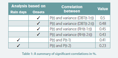
To obtain a statistical relationship between precipitation and other weather elements, we perform a correlation analysis which is explained in detail in a previous study [13] and all significant correlations are summarised in Table 1.
Monte Carlo Markov Chain model using simulated annealing
In this section, we present a Monte Carlo Markov chain (MCMC) model to exploit the high correlations between precipitation onsets and other weather elements. MCMC-based models do not utilise the probabilistic information but rather they directly use the observed properties of the precipitation series, such as the correlation between precipitation onsets and other weather elements [12].
The states of the MCMC model in this case are defined on the set of possible precipitation time series, not as a sample from a probabilistic model. To generate the synthesised precipitation series, an optimisation technique called simulated annealing introduced by Kirkpatrick et al. in 1983 [14] is utilised. The simulated annealing optimisation works on the Metropolis-Hastings algorithm, where the objective function aims to minimise the differences between the properties of the generated series and the corresponding observed dataset.
In the MCMC model, hourly precipitation series is modelled as a random vector
P = [P(1), P(2), …, P(T)] ∈ RT P = [P(1), P(2), …, P(T)] ∈ RT
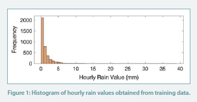
where T is the length of the series (or total number of under-study hours). All possible values for each element of this vector can be obtained using the observed historical data. For instance, all the possible hourly precipitation values for Canberra, using the training dataset (a dataset of several years with both half-hourly and daily precipitation used to facilitate machine learning of their statistical association), include
{0, 0.2, … , 36.8}{0, 0.2, … , 36.8}
millimeter (mm).
Therefore, the precipitation of each timestamp has 194 possible values and thus the total possible precipitation series for T timestamps is 194T. Note that assessing all possible series when T is a large number (e.g., hourly for one year or more as is typical for building simulations) is practically impossible. Instead, we can only consider two possible series namely P1 and P2 and assign the conditional probabilities to them:
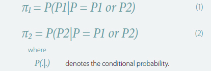
where P(.|.) denotes the conditional probability. We then utilise the Metropolis-Hastings algorithm, which is an MCMC method for obtaining a sequence of random samples from a probability distribution from which direct sampling is difficult [14]. Based on this algorithm, an acceptance ratio is defined for the two considered series P1 and P2, as follows:

If the acceptance ratio α21 is great than 1, which means the probability π2 is greater than π1, we choose series P2 over the other candidate, i.e., P1. This is because π2 > π1 shows that the series P2 is more probable to be the desired precipitation series compared to the series P1. However, if α21 ≤ 1 then a uniform random number u ∈ [0, 1] is generated and by comparing the acceptance ratio α21 with u, the algorithm decides to either accept or reject each candidate. In summary:

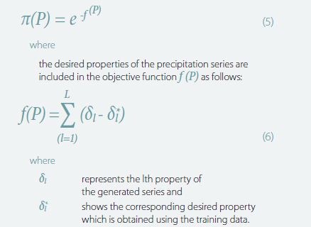
To assign the probabilities π1 and π2, we need to define the desired properties of the precipitation series. For this purpose, we use the simulated annealing approach where these probabilities are defined using an objective function (f) which depends on the corresponding series. Therefore, the probability of a given precipitation series P is defined as follows:
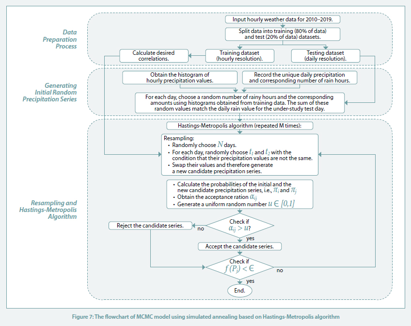
SIMULATED ANNEALING TECHNIQUE BASED ON HASTINGS-METROPOLIS ALGORITHM
Aerosol testing was conducted in the classroom to assess validity of the well-mixed assumption in the Wells-Riley model. A polydisperse neutralised salt (NaCl) in an aerosol size range consistent with human-generated bioaerosols containing SARS-CoV-2 was used as a safe surrogate for respiratory droplets or quanta. Although the target aerosol particle size for the study was 200nm to 5μm, the aerosol actually produced and dispersed into the classroom spanned a range of 100nm to 8μm, with the measured distribution shown in Figure 4.
A single manikin at the location indicated by the green dot in Figure 2 was set up to “exhale” aerosol into the room, while the remaining manikins were set up to “inhale” so that the local aerosol concentration could be measured. Figure 5 shows the measured distribution of aerosol concentration for two different aerodynamic diameters, 0.728μm (a) and 2.71μm (b). The aerosol concentration is normalised by the lowest concentration in the room for each diameter and case shown. The normalised concentration distribution for the 0.728μm aerosol size was generally more uniform than that for the 2.71μm size. Not surprisingly, the normalised aerosol concentration near the source trended higher in both cases.
Additional tests were conducted with manikins being equipped with masks, and similar aerosol distribution trends were noted. The greater nonuniformity in aerosol concentration for the larger size suggests that a higher fraction of the larger particles settled rather than being transported throughout the room on air currents, as was the case for the smaller 0.728μm size aerosols. This result implies that smaller particle sizes may be more uniformly distributed in the room and that the well-mixed assumption may hold better for particle sizes in this general size range. Further details on the aerosol dynamics for this space are provided by Rothamer, et al.
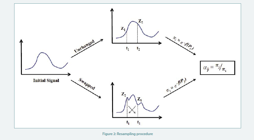
The next step is to generate another candidate for the precipitation series using resampling. For this purpose, we randomly choose d days and for each day, two times t1 ̸= t2 are selected to swap their hourly rain values. Note that swapping is done with the condition that the amount of hourly rain values is different for the selected times. This process is called resampling and generates a new time series.
To accept or reject the new candidate the probability of the two series is calculated using (5) and (6). Then, the acceptance ratio (3) is calculated and based on the criterion (5), the algorithm decides either accept or reject the new candidate. This procedure is demonstrated Figure 2. The resampling process is repeated for M times. The algorithm will stop when the stopping criterion f (P) ≤ ϵ is reached.
Results
In this section, we perform six different experiments taking the significant correlations in Table 1 into account and using the MCMC model. The experiments include:
1) P (Lag1): considering only Lag 1 of the precipitation and
2) P (Lags 1, 2): considering Lag 1 and Lag 2 of the precipitation,
3) Var (RH1): considering variance of relative humidity during the past hour,
4) Var (RH2): considering variance of relative humidity during the past two hours,
5) Var (DBT1): considering variance of dew point temperature during the past hour, and
6) Var (DBT2): considering variance of dew point temperature during the past two hours.
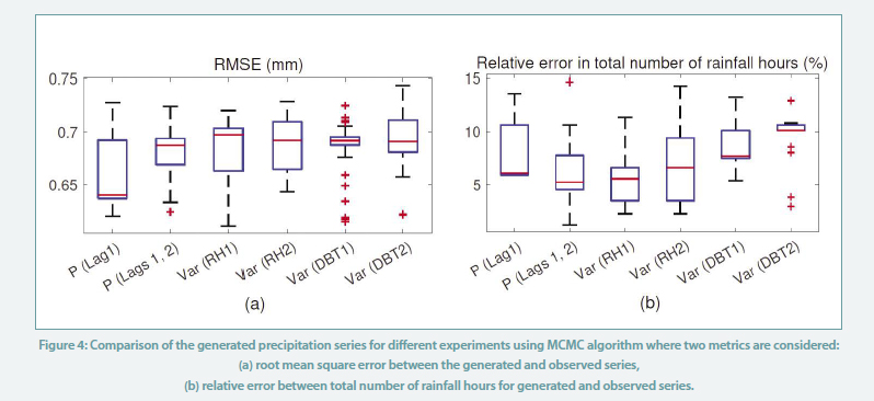
We repeat the MCMC algorithm 100 times to account for the uncertain nature of this algorithm. We calculate the RMSE between the generated and the actual precipitation series. The boxplot is shown in Figure 4 (a) demonstrates this RMSE for all the experiments. Also, the relative error between the total number of rainfall hours in the generated series with the corresponding number in the observed series is shown in Figure 4 (b).
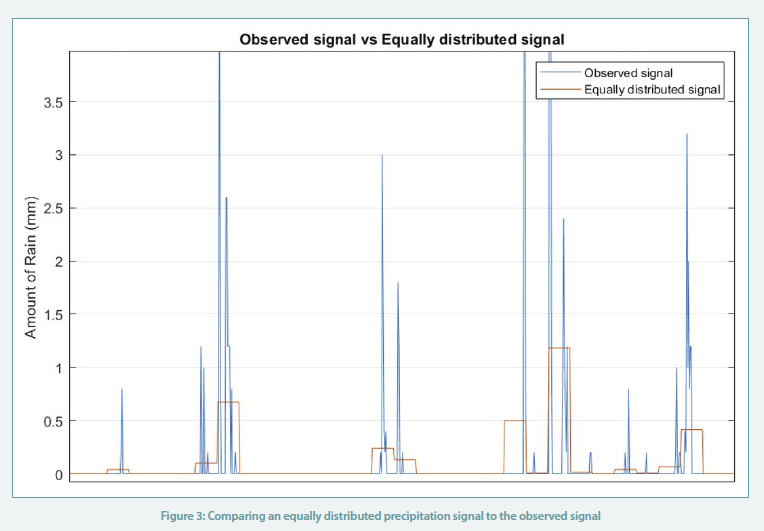
We observe that the RMSEs obtained using MCMC algorithm are two times less than the error of the series obtained using the simple Markov chain algorithm (errors ~0.7 compared to error ~1.4). In comparison, if we equally distribute the daily precipitation across the 24 hours as shown in Figure 3, the resulting RMSE obtained is around 0.9, implying a higher deviation from the observed readings.
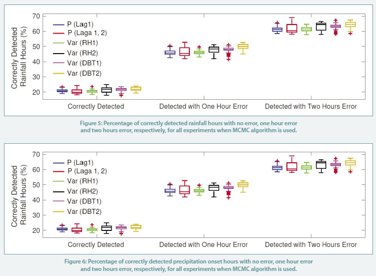
In addition to these metrics, the number of correctly detected rainfall hours and correctly detected precipitation onset hours are obtained as shown in Figure 5 and Figure 6 , respectively. We observe that the MCMC algorithm detects at least 60% of the rainfall hours with less than two hours error. It also detects at least 50% of the precipitation onset hours with the same error.
Conclusion
This paper develops a stochastic algorithm based on Markov chain Monte Carlo (MCMC) methods to generate hourly temporal resolution precipitation data in Australian locations based on the daily precipitation data recorded by the Bureau of Meteorology (BoM) before 2000. The proposed algorithms use a combination of data recorded for weather elements like temperature, relative humidity and cloud cover, along with the precipitation data.
The generated synthesised hourly precipitation series are compared with the observed series using three metrics including 1) least-square residuals, 2) the total number of rain hours, and 3) the total number of matching onset hours between the generated and observed precipitation series. We observe improvements in the considered metrics when the other weather elements are integrated in the developed algorithms.
Based on the results obtained for the MCMC algorithm, when considering only precipitation with an hour lag, the least deviation from the actual series was obtained. When considering other weather elements, the addition of relative humidity with an hour lag shows promising results. This model is intended to be expanded to include different climate zones of Australia and, if successful, will be used to include precipitation data from 1990 to the present, to the weather and climate data of over 250 Australian locations which Exemplary Energy produces. Thus, the precipitation data in these weather data, being present for over 30 years, will fulfill the condition of a climate normal as per WMO and can be reliably used for modelling and simulations of varied nature in the built environment domain.
To improve the accuracy of the generated synthetic signals, some of the avenues that will be investigated in the future include: 1) effects of implementing raw data with half-hourly resolution, and 2) the impact of segregating the training and testing data by seasonality.
References
| [1] | T. Asim, R. Mishra, S. Rodrigues and B. Nsom, “Applications of Numerical Simulations in Built,” International Journal of COMADEM, vol. 22, p. 9–14, 2019. |
| [2] | Y. Lai and D. Dzombak, “Use of Historical Data to Assess Regional Climate Change,” Journal of Climate, vol. 32, p. 4299–4320, 2019. |
| [3] | Australian government, “B.O.M. Observation of Rainfall,” 2010. [Online]. Available: http://www.bom.gov.au/climate/how/measure.shtml. |
| [4] | G. Brigandì and G. Aronica, “Generation of Sub-Hourly Rainfall Events through a Point Stochastic Rainfall Model,” Geosciences, vol. 9, 2019. |
| [5] | F. Lombardo, E. Volpi, D. Koutsoyiannis and F. Serinaldi, “A theoretically consistent stochastic cascade for temporal disaggregation of intermittent rainfall.,” Water Resources Research, vol. 53, p. 4586–4605, 2017. |
| [6] | L. Guenni and A. Bárdossy, “A two steps disaggregation method for highly seasonal monthly rainfall,” Stochastic Environmental Research and Risk Assessment (SERRA), vol. 16, p. 88–206, 2002. |
| [7] | C. Miao, J. Chen, J. Liu and H. Su, “An improved Markov chain model for hour-ahead wind speed prediction.,” 2015 34th Chinese Control Conference (CCC), p. 8252–8257, 2015. |
| [8] | C. Onof, R. Chandler, A. Kakou, P. Northrop, H. Wheater and V. Isham, “Rainfall modelling using Poisson-cluster processes: a review of developments.,” Stochastic Environmental Research and Risk Assessment, vol. 14, p. 0384–0411, 2000. |
| [9] | P. Cowpertwait, V. Isham and C. Onof, “Point process models of rainfall: developments for fine-scale structure.,” Proceedings of the Royal Society A: Mathematical, Physical and Engineering Sciences, vol. 463, p. 2569–2587, 2007. |
| [10] | R. Srikanthan, T. Harrold, A. Sharma and T. Mcmahon, “Comparison of two approaches for generation of daily rainfall data.,” Stochastic Environmental Research and Risk Assessment, vol. 19, p. 215–226, 2005. |
| [11] | Y. Zou, Z. Kong, T. Liu and D. Liu, “A Real-Time Markov Chain Driver Model for Tracked Vehicles and Its Validation: Its Adaptability via Stochastic Dynamic Programming.,” IEEE Transactions on Vehicular Technology, vol. 66, p. 3571–3582, 2017. |
| [12] | A. Bárdossy, “Generating precipitation time series using simulated annealing,” Water Resources Research, vol. 34, p. 1737–1744, 1998. |
| [13] | D. Ferrari, M. Mahmoodi, C. Kodagoda, N. Abdul Hameed, T. Lee and G. Anderson, “Temporal Disaggregation of Precipitation Data Applicable for Climate-aware Planning in Built Environments,” in Asia Solar Pacific Conference, Sydney, 2021. |
| [14] | S. Kirkpatrick, C. Gelatt and M. Vecchi, “Optimization by simulated annealing,” science, vol. 220, p. 671–680, 1983. |
Acknowledgements
The authors acknowledge the Australian Bureau of Meteorology as the source of all the raw data, the College of Engineering and Computer Science, Australian National University, and the other members of the Exemplary team.

This article appears in Ecolibrium’s April 2023 edition
View the archive of previous editions


Latest edition
See everything from the latest edition of Ecolibrium, AIRAH’s official journal.